
Integrated Computational Materials Engineering (ICME)
Making Stress-Strain Plots with MATLAB
Abstract
This example shows how to plot a stress-strain curve in MATLAB using output data from the parallel molecular dynamics code, LAMMPS. This example will reference the scripts and data of the Uniaxial Tension in Single Crystal Aluminum and Uniaxial Compression in Single Crystal Aluminum examples.
Author(s): Nathan R. Rhodes, Mark A. Tschopp
LAMMPS Input
In order to have LAMMPS output data useful for plotting, the simulation cell length must be stored; and the stress and strain data must be written to an external file.The following script shows how the final cell length is stored in the aluminum examples. The cell length is lx, while the initial length of the cell is stored as L0. These values are needed for strain calculation. Note that these commands are written before deformation commands in the input scripts.
# Store final cell length for strain calculations
variable	tmp equal "lx"
variable	L0 equal ${tmp}
variable	L0 equal 40.64912642
print		"Initial Length, L0: ${L0}"
Initial Length, L0: 40.64912642
The following script shows how the aluminum examples write stress and strain data to a file. Strain is calculated from variables defined above and is stored as p1. The principal stresses are first converted to GPa and then stored as p1, p2, and p3. The fix command is used to print these four variables to a new file, in this case, named "Al_comp.def1.txt." When LAMMPS is run, this file appears in the directory with other LAMMPS output files. Note that these commands are written after the deformation procedure in the input scripts.
# Output strain and stress information to file.
# For metal units, pressure is [bars] = 100 [kPa] = 1/10000 [GPa]
# p2, p3, and p4 are in GPa

variable 		strain equal "(lx - v_L0) / v_L0"
variable 		p1 equal "v_strain"
variable 		p2 equal "-pxx/10000"
variable 		p3 equal "-pyy/10000"
variable 		p4 equal "-pzz/10000"
fix 		def1 all print 100 "${p1} ${p2} ${p3} ${p4}" file Al_comp.def1.txt screen no
LAMMPS Datafiles
The following datafiles were created for the tension and compression aluminum examples.
Al_SC_100.def1.txt:
# Fix print output for fix def1
0.0009999999119 0.08667300618 0.03175758225 0.03801213452
0.001999999912 0.09131420312 -0.05499624531 -0.03396621651
0.002999999912 0.2254889267 0.04825004506 0.04680554658
0.003999999912 0.2199842183 -0.04156649661 -0.02074145126
0.004999999912 0.3127067321 0.01435171918 0.01093418588
...
Al_comp.def1.txt:
# Fix print output for fix def1
-0.001000000088 -0.06084024339 0.005103309452 0.011634529
-0.002000000088 -0.1414344573 -0.02482512452 -0.00442782696
-0.003000000088 -0.1893439523 0.009944994037 0.01031293284
-0.004000000088 -0.2745471681 -0.01431999273 0.006837682636
-0.005000000088 -0.3417247015 -0.005247107989 -0.01437892764
...
MATLAB Script
The stress strain curve for the aluminum in tension and compression examples can be seen in Figures 1 and 2. The following MATLAB script will plot the stress-strain curve for either case, provided the LAMMPS datafile and this script are located in the same directory. Note that values are negative in the compressive case. In order to attain the image in Figure 2, simply make negative the strain and stress variables in the script.
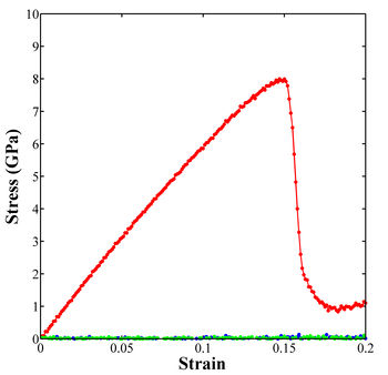
Figure 1. Stress-strain curve for uniaxial tensile loading of single crystal aluminum in the <100> loading direction.
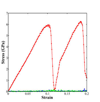
Figure 2. Stress-strain curve for uniaxial compressive loading of single crystal aluminum in the <100> loading direction.
The plot can be saved as a MATLAB figure after it appears. Additionally, the exportfig command, which refers to a script that can be downloaded at the MATLAB Central File website, exports the plot to a tiff file.
%% Analyze def1.txt files
% Plot the various responses

d = dir('*.def1.txt');
for i = 1:length(d)
    % Get data
    fname = d(i).name;
    A = importdata(fname);
    % Define strain as first column of data in A (*.def1.txt)
    strain = A.data(:,1);
    % Define stress as second through fourth columns in A (*def1.txt)
    stress = A.data(:,2:4);

    % Generate plot
    plot(strain,stress(:,1),'-or','LineWidth',2,'MarkerEdgeColor','r',...
                'MarkerFaceColor','r','MarkerSize',5),hold on
    plot(strain,stress(:,2),'-ob','LineWidth',2,'MarkerEdgeColor','b',...
                'MarkerFaceColor','b','MarkerSize',5),hold on
    plot(strain,stress(:,3),'-og','LineWidth',2,'MarkerEdgeColor','g',...
                'MarkerFaceColor','g','MarkerSize',5),hold on
    axis square
    ylim([0 10])
    set(gca,'LineWidth',2,'FontSize',24,'FontWeight','normal','FontName','Times')
    set(get(gca,'XLabel'),'String','Strain','FontSize',32,'FontWeight','bold','FontName','Times')
    set(get(gca,'YLabel'),'String','Stress (GPa)','FontSize',32,'FontWeight','bold','FontName','Times')
    set(gcf,'Position',[1 1 round(1000) round(1000)])

    % Export the figure to a tif file
    exportfig(gcf,strrep(fname,'.def1.txt','.tif'),'Format','tiff',...
        'Color','rgb','Resolution',300)

end
The following script will combine the tensile and compressive curves into a single plot, seen in Figure 3. Note that only the principal stresses in the x direction have been included.
% Compare responses for Uniaxial Tension and Compression in Single Crystal
% Aluminum

%Find files from which to pull data
a = dir('Al_SC_100.def1.txt');
b = dir('Al_comp.def1.txt');
for i = 1:length(a)

    %Pull data and define columns and stress and strain
    fname_t = a(i).name;
    A = importdata(fname_t);
    strain_t = A.data(:,1);
    stress_t = A.data(:,2);

    fname_c = b(i).name;
    B = importdata(fname_c);
    strain_c = -B.data(:,1);
    stress_c = -B.data(:,2);

    %Plot columns of data on a common graph
    plot(strain_t,stress_t,'-or','LineWidth',2,'MarkerEdgeColor','r',...
        'MarkerFaceColor','r','MarkerSize',5),hold on
    plot(strain_c,stress_c,'-ob','LineWidth',2,'MarkerEdgeColor','b',...
        'MarkerFaceColor','b','MarkerSize',5),hold on
    axis square
    ylim([0,9])

    %Configure labels for the axes
    set(gca,'LineWidth',2,'FontSize',12,'FontWeight','normal','FontName','Times')
    set(get(gca,'xlabel'),'String','Strain','FontSize',20,'FontWeight','bold','FontName','Times')
    set(get(gca,'ylabel'),'String','Stress (GPa)','FontSize',20','FontWeight','bold','FontName','Times')
    set(gcf,'Position',[1 1 round(1000) round(1000)])

    %Display a legend to label the curves
    legend('show','Tension','Compression')

    % Export the figure to a tif file
    exportfig(gcf,strrep(fname_t,'Al_SC_100.def1.txt','jointfig.tif'),'Format','tiff',...
        'Color','rgb','Resolution',300)
end
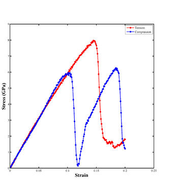
Figure 3. Stress-strain curve for uniaxial tensile and compressive loading of single crystal aluminum in the <100> direction.