
Integrated Computational Materials Engineering (ICME)
Uniaxial Compression
Abstract
This example shows how to run an atomistic simulation of uniaxial compressive loading of an aluminum single crystal oriented in the <100> direction. It also compares results of simulations with 4,000, 32,000, and 108,000 atoms. This example uses a parallel molecular dynamics code, LAMMPS[1]. These scripts were initially used to study dislocation nucleation in single crystal aluminum and copper[2][3][4].
Author(s): Mark A. Tschopp, Nathan R. Rhodes
Input
Description of Simulation
This molecular dynamics simulation first generates a simulation cell with fcc atoms with <100> orientations in the x, y, and z-directions. For this example, the simulation cell size is 10 lattice units in each direction for 4,000 total atoms, 20 units for 32,000 atoms, and 30 units for 108,000 atoms. Larger simulation cell sizes should be used to converge the dislocation nucleation stress values and to not influence the dislocation nucleation mechanism. The potential used in the Mishin et al. (1999) aluminum potential[5]. The equilibration step allows the lattice to expand to a temperature of 300 K with a pressure of 0 bar at each simulation cell boundary. Then, the simulation cell is deformed in the x-direction at a strain rate of 1010 s-1, while the lateral boundaries are controlled using the NPT equations of motion to zero pressure. The stress and strain values are output to a separate file, which can be imported in a graphing application for plotting. The cfg dump files include the x, y, and z coordinates, the centrosymmetry values, the potential energies, and forces for each atom. This can be directly visualized using AtomEye[6].
Movie showing compressive deformation of single crystal of 108,000 aluminum atoms loaded in the <100> direction at a strain rate of 1010 s-1 and a temperature of 300 K.
LAMMPS input script
This input script was run using the Aug 2015 version of LAMMPS. Changes in some commands in more recent versions may require revision of the input script. This script runs the simulation with 4,000 atoms. To change the number of atoms, alter the numbers (currently 10) after the "region" command under "Atom Definition." To run this script, store it in "in.comp.txt" and then use "lmp_exe < in.comp.txt" in a UNIX environment where "lmp_exe" refers to the LAMMPS executable.
Notice that the only difference, besides file names, between this script and the script for uniaxial tension is the negative in the definition of variable "srate1."
# Input file for uniaxial compressive loading of single crystal aluminum
# Mark Tschopp, November 2010

# ------------------------ INITIALIZATION ----------------------------
units 		metal
dimension	3
boundary	p	p	p
atom_style	atomic
variable latparam equal 4.05

# ----------------------- ATOM DEFINITION ----------------------------
lattice		fcc ${latparam}
region		whole block 0 10 0 10 0 10
create_box	1 whole

region		upper block INF INF INF INF INF INF units box
lattice 	fcc ${latparam} orient x 1 0 0 orient y 0 1 0 orient z 0 0 1
create_atoms	1 region upper

# ------------------------ FORCE FIELDS ------------------------------
pair_style	eam/alloy
pair_coeff	* * Al99.eam.alloy Al

# ------------------------- SETTINGS ---------------------------------
compute csym all centro/atom fcc
compute peratom all pe/atom

######################################
# EQUILIBRATION
reset_timestep	0
timestep 0.001
velocity all create 300 12345 mom yes rot no
fix 1 all npt temp 300 300 1 iso 0 0 1 drag 1

# Set thermo output
thermo 1000
thermo_style custom step lx ly lz press pxx pyy pzz pe temp

# Run for at least 10 picosecond (assuming 1 fs timestep)
run 20000
unfix 1

# Store final cell length for strain calculations
variable tmp equal "lx"
variable L0 equal ${tmp}
print "Initial Length, L0: ${L0}"

######################################
# DEFORMATION
reset_timestep	0

fix		1 all npt temp 300 300 1 y 0 0 1 z 0 0 1 drag 1
variable srate equal 1.0e10
variable srate1 equal "-v_srate / 1.0e12"
fix		2 all deform 1 x erate ${srate1} units box remap x

# Output strain and stress info to file
# for units metal, pressure is in [bars] = 100 [kPa] = 1/10000 [GPa]
# p2, p3, p4 are in GPa
variable strain equal "(lx - v_L0)/v_L0"
variable p1 equal "v_strain"
variable p2 equal "-pxx/10000"
variable p3 equal "-pyy/10000"
variable p4 equal "-pzz/10000"
fix def1 all print 100 "${p1} ${p2} ${p3} ${p4}" file Al_comp_100.def1.txt screen no

# Use cfg for AtomEye
dump 		1 all cfg 250 dump.comp_*.cfg mass type xs ys zs c_csym c_peratom fx fy fz
dump_modify     1 element Al

# Display thermo
thermo 	1000
thermo_style	custom step v_strain temp v_p2 v_p3 v_p4 ke pe press

run		20000

######################################
# SIMULATION DONE
print "All done"
Output
LAMMPS logfile
The log.lammps file should look like this below. Notice that the 20 ps (20,000 fs) equilibration step brought the temperature of the simulation cell up to 300 K. The corresponding deformation went up to a strain of 0.2. The thermo command was set for every 1000 timesteps, so any plots should be made from the data included in the datafile.
LAMMPS (5 Nov 2010)
# Input file for uniaxial compressive loading of single crystal aluminum
#Mark Tschopp, November 2010

# ----- INITIALIZATION -----
units		metal
dimension	3
boundary	p	p	p
atom_style	atomic
variable 		latparam equal 4.05

# ----- ATOM DEFINITION -----
lattice		fcc ${latparam}
lattice		fcc 4.05
Lattice spacing in x,y,z = 4.05 4.05 4.05
region		whole block 0 10 0 10 0 10
create_box	1 whole
Created orthogonal box = (0 0 0) to (40.5 40.5 40.5)
  2 by 2 by 2 processor grid

region		upper block INF INF INF INF INF INF units box
lattice		fcc ${latparam} orient x 1 0 0 orient y 0 1 0 orient z 0 0 1
lattice		fcc 4.05 orient x 1 0 0 orient y 0 1 0 orient z 0 0 1
Lattice spacing in x,y,z = 4.05 4.05 4.05
create_atoms	1 region upper
Created 4000 atoms

# ----- FORCE FIELDS -----
pair_style	eam/alloy
pair_coeff	* * Al99.eam.alloy Al

# -----SETTINGS -----
compute	csym all centro/atom fcc
compute	peratom all pe/atom

# ----- EQUILIBRATION -----
reset_timestep	0
timestep	0.001
velocity	all create 300 12345 mom yes rot no
fix		1 all npt temp 300 300 1 iso 0 0 1 drag 1

# Set Thermo Input
thermo		1000
thermo_style	custom step lx ly lz press pxx pyy pzz pe temp

# Run Time (At least 10 picoseconds)
run		20000
Memory usage per processor = 2.55571 Mbytes
Step Lx Ly Lz Press Pxx Pyy Pzz PotEng Temp
       0         40.5         40.5         40.5    2496.1233    2446.9902    2534.6541    2506.7256       -13440          300
    1000    40.558342    40.558342    40.558342    731.50829    755.55351    696.37101    742.60035   -13363.301    169.49172
    2000    40.574199    40.574199    40.574199    106.78935   -46.253007    296.26883    70.352219   -13356.097    178.17311
    3000    40.579471    40.579471    40.579471    314.81803    314.71612    292.22553    337.51245   -13347.025      183.623
    4000    40.586697    40.586697    40.586697    107.84524    52.829414    112.73441     157.9719   -13340.823    194.61149
    5000    40.593224    40.593224    40.593224    172.67874    158.86784    199.13978    160.02861   -13334.364    204.85854
    6000    40.601567    40.601567    40.601567    56.953653   -6.2830484   -16.301111    193.44512    -13327.55    213.93605
    7000     40.60782     40.60782     40.60782    31.891969    35.437938    63.396951   -3.1589825    -13320.86    222.48071
    8000    40.616908    40.616908    40.616908   -244.41321   -212.11716   -305.70692   -215.41555   -13317.384      236.254
    9000    40.618876    40.618876    40.618876    13.561356    111.07353   -29.999797   -40.389663   -13313.071    247.18002
   10000    40.625506    40.625506    40.625506   -125.06329    -105.4566   -93.514599   -176.21866   -13308.875    256.93613
   11000    40.631525    40.631525    40.631525   -75.690987    141.36136    14.068057   -382.50238   -13303.582    263.00631
   12000    40.631815    40.631815    40.631815     79.38005    63.796397    144.76416    29.579595    -13299.23    269.23326
   13000    40.637408    40.637408    40.637408    -152.9113   -399.37081   -31.484802   -27.878283   -13298.162     280.0582
   14000    40.636962    40.636962    40.636962    237.09239    58.799334    196.78768    455.69014   -13294.166    283.43969
   15000    40.641455    40.641455    40.641455    105.44503    114.55343     142.4659    59.315739   -13291.527    287.73561
   16000    40.643072    40.643072    40.643072    82.986611   -130.36308     288.9926    90.330318   -13288.384    289.39655
   17000     40.64789     40.64789     40.64789   -12.310673   -112.67891    -132.8659     208.6128   -13289.081    296.89271
   18000    40.644319    40.644319    40.644319    269.36896    180.82571    218.97472    408.30644   -13286.862    297.25615
   19000    40.646772    40.646772    40.646772    166.57104    20.881491   -79.807885    558.63952   -13287.577    301.80321
   20000    40.649126    40.649126    40.649126    116.57534   -108.86953    156.54682    302.04873   -13284.646    298.01867
Loop time of 79.3677 on 8 procs for 20000 steps with 4000 atoms

Pair  time (%) = 63.798 (80.3828)
Neigh time (%) = 0 (0)
Comm  time (%) = 12.2773 (15.4689)
Outpt time (%) = 0.00290701 (0.00366271)
Other time (%) = 3.28956 (4.1447)

Nlocal:    500 ave 500 max 500 min
Histogram: 8 0 0 0 0 0 0 0 0 0
Nghost:    2930 ave 2930 max 2930 min
Histogram: 8 0 0 0 0 0 0 0 0 0
Neighs:    35000 ave 36430 max 33540 min
Histogram: 2 0 1 1 0 0 1 1 0 2
FullNghs: 0 ave 0 max 0 min
Histogram: 8 0 0 0 0 0 0 0 0 0

Total # of neighbors = 280000
Ave neighs/atom = 70
Neighbor list builds = 0
Dangerous builds = 0
unfix		1

# Store final cell length for strain calculations
variable	tmp equal "lx"
variable	L0 equal ${tmp}
variable	L0 equal 40.64912642
print		"Initial Length, L0: ${L0}"
Initial Length, L0: 40.64912642

# -----DEFORMATION -----
reset_timestep	0
fix		1 all npt temp 300 300 1 y 0 0 1 z 0 0 1 drag 1
variable	srate equal 1e10

#The only difference between this compressive example and
#the previous tensile example is the negative sign in the
#definition of srate1, seen below.

variable	srate1 equal "-v_srate / 1e12"
fix		2 all deform 1 x erate ${srate1} units box remap x
fix		2 all deform 1 x erate -0.01 units box remap x

# Output strain and stress information to file.
# For metal units, pressure is [bars] = 100 [kPa] = 1/10000 [GPa]
# p2, p3, and p4 are in GPa

variable 		strain equal "(lx - v_L0) / v_L0"
variable 		p1 equal "v_strain"
variable 		p2 equal "-pxx/10000"
variable 		p3 equal "-pyy/10000"
variable 		p4 equal "-pzz/10000"
fix 		def1 all print 100 "${p1} ${p2} ${p3} ${p4}" file Al_comp.def1.txt screen no

# Dump to cfg for AtomEye post processing
dump		1 all cfg 250 dump.comp_*.cfg id type xs ys zs c_csym c_peratom fx fy fz
dump_modify	1 element Al

# Display thermo information
thermo		1000
thermo_style	custom step v_strain temp v_p2 v_p3 v_p4 ke pe press

run		20000
Memory usage per processor = 2.8622 Mbytes
Step strain Temp p2 p3 p4 KinEng PotEng Press
       0 -8.7965858e-11    298.01867  0.010886953 -0.015654682 -0.030204873    154.04923   -13284.646    116.57534
    1000        -0.01    302.82586  -0.61033601  0.054190295 -0.0032380699    156.53411   -13286.645    1864.6126
    2000        -0.02    298.61071   -1.2849368  -0.00313581  0.026906426    154.35526   -13281.302    4203.8871
    3000        -0.03    302.18611   -1.8380212 -0.011375474 0.0087206074    156.20342   -13277.349    6135.5869
    4000        -0.04    297.31028   -2.4628066 -0.0095117003 -0.026443669    153.68305   -13266.262    8329.2065
    5000        -0.05    294.28788   -3.0927297 -0.0021071467 -0.050407399    152.12073   -13253.309    10484.147
    6000        -0.06     301.6804   -3.7194292  -0.01909606  0.018996497    155.94201   -13242.696    12398.429
    7000        -0.07    298.64768   -4.4073614  0.019050091  0.051288755    154.37437   -13223.403    14456.742
    8000        -0.08    298.53159   -5.0314374  0.046526108 0.0042843939    154.31436   -13202.054     16602.09
    9000        -0.09    289.63258   -5.5876729 0.0064037479   0.07394267    149.71436   -13172.278    18357.755
   10000         -0.1    284.07377   -5.8774427  0.011876434  0.017658887    146.84095   -13140.895    19493.024
   11000        -0.11    320.11761   -4.2791145  0.062847323  0.072604489    165.47242   -13130.428    13812.209
   12000        -0.12    384.47793  -0.26899312   0.06384105  0.075858441    198.74099   -13172.063    430.97876
   13000        -0.13     406.8698   -2.3913058 -0.036697295 -0.037783423    210.31561    -13200.26    8219.2883
   14000        -0.14    385.84693   -3.3014902  0.059581512 -0.048723245    199.44864   -13199.524    10968.773
   15000        -0.15    365.16317   -4.0204884  0.058056622  0.017209135    188.75697   -13191.173    13150.742
   16000        -0.16    352.29941   -4.8141755  0.052769795 -0.039907224    182.10755   -13179.442    16004.377
   17000        -0.17    333.83554   -5.4774396  0.014373592 -0.0069549415    172.56337    -13157.84    18233.403
   18000        -0.18     326.9576   -6.0482935  0.022646093  0.050253999    169.00809   -13135.624    19917.978
   19000        -0.19    328.65703   -5.4349022 -0.052976878   0.02948022    169.88654   -13113.032    18194.663
   20000         -0.2     402.8138   -1.2165489  0.030833241 -0.037641657    208.21901   -13158.984    4077.8578
Loop time of 95.4143 on 8 procs for 20000 steps with 4000 atoms

Pair  time (%) = 74.0979 (77.6591)
Neigh time (%) = 0.127079 (0.133187)
Comm  time (%) = 11.7939 (12.3607)
Outpt time (%) = 2.51201 (2.63274)
Other time (%) = 6.8834 (7.21423)

Nlocal:    500 ave 507 max 495 min
Histogram: 2 1 0 0 2 1 1 0 0 1
Nghost:    2485.88 ave 2494 max 2479 min
Histogram: 1 1 2 0 1 0 0 1 0 2
Neighs:    35096 ave 36398 max 34125 min
Histogram: 2 0 2 1 0 0 0 2 0 1
FullNghs: 70196.5 ave 71230 max 69522 min
Histogram: 3 0 0 0 2 1 1 0 0 1

Total # of neighbors = 561572
Ave neighs/atom = 140.393
Neighbor list builds = 62
Dangerous builds = 0

print "All done"
All done
LAMMPS datafile
The following datafile, Al_comp.def1.txt, was also generated during this simulation.
# Fix print output for fix def1
-0.001000000088 -0.06084024339 0.005103309452 0.011634529
-0.002000000088 -0.1414344573 -0.02482512452 -0.00442782696
-0.003000000088 -0.1893439523 0.009944994037 0.01031293284
-0.004000000088 -0.2745471681 -0.01431999273 0.006837682636
-0.005000000088 -0.3417247015 -0.005247107989 -0.01437892764
-0.006000000087 -0.3715769192 0.03762760787 0.03762638331
-0.007000000087 -0.4593169714 -0.03208865692 0.002251496376
-0.008000000087 -0.5124145984 0.00431254376 0.04566519111
...
LAMMPS dumpfile
The following is the beginning of one of the dumpfiles in cfg format that were also generated during this simulation.
Number of particles = 4000
A = 1.0 Angstrom (basic length-scale)
H0(1,1) = 40.6491 A
H0(1,2) = 0 A
H0(1,3) = 0 A
H0(2,1) = 0 A
H0(2,2) = 40.6491 A
H0(2,3) = 0 A
H0(3,1) = 0 A
H0(3,2) = 0 A
H0(3,3) = 40.6491 A
.NO_VELOCITY.
entry_count = 8
auxiliary[0] = csym
auxiliary[1] = peratom
auxiliary[2] = fx
auxiliary[3] = fy
auxiliary[4] = fz
26.982
Al
0.0493442 0.0581882 0.00323696 1.58804 -3.34266 0.196691 -0.804728 -0.0280286
0.0987502 0.00417997 0.00238952 0.827133 -3.34273 -0.475844 -0.270217 -0.120716
0.0989802 0.0523976 0.0521907 0.363772 -3.30304 -0.309005 -0.274515 -0.299433
0.0495058 0.102418 0.0536544 0.611128 -3.30518 0.162097 -0.42069 -0.15808
0.0995051 0.102793 0.00119416 0.614289 -3.28181 -0.406727 -0.192102 0.405813
0.0473774 0.0488825 0.10204 0.581043 -3.3709 0.135458 -0.205472 -0.294232
0.0989535 0.000697083 0.0977144 0.583569 -3.30702 -0.474259 0.0845695 0.400838
...
Post-Processing
Stress-Strain Plot
The stress-strain curve in Figure 1 can be generated using the following MATLAB script. Note that the definitions of stress and strain are negative. This is done to counteract the negative values of compressive stress and strain so that positive axes and a familiar shape are retained. The "exportfig" command saves the plot to a tiff files, but the plot can also be saved as a Mathcad figure once it appears.
%% Analyze def1.txt files
% Plot the various responses

d = dir('*.def1.txt');
for i = 1:length(d)
    % Get data
    fname = d(i).name;
    A = importdata(fname);
    strain = A.data(:,1);
    stress = A.data(:,2:4);

    % Generate plot
    plot(strain,stress(:,1),'-or','LineWidth',2,'MarkerEdgeColor','r',...
                'MarkerFaceColor','r','MarkerSize',5),hold on
    plot(strain,stress(:,2),'-ob','LineWidth',2,'MarkerEdgeColor','b',...
                'MarkerFaceColor','b','MarkerSize',5),hold on
    plot(strain,stress(:,3),'-og','LineWidth',2,'MarkerEdgeColor','g',...
                'MarkerFaceColor','g','MarkerSize',5),hold on
    axis square
    ylim([0 10])
    set(gca,'LineWidth',2,'FontSize',24,'FontWeight','normal','FontName','Times')
    set(get(gca,'XLabel'),'String','Strain','FontSize',32,'FontWeight','bold','FontName','Times')
    set(get(gca,'YLabel'),'String','Stress (GPa)','FontSize',32,'FontWeight','bold','FontName','Times')
    set(gcf,'Position',[1 1 round(1000) round(1000)])

    % Export figure to tif file
    exportfig(gcf,strrep(fname,'.def1.txt','.tif'),'Format','tiff',...
    'Color','rgb','Resolution',300)
    close(1)

    end
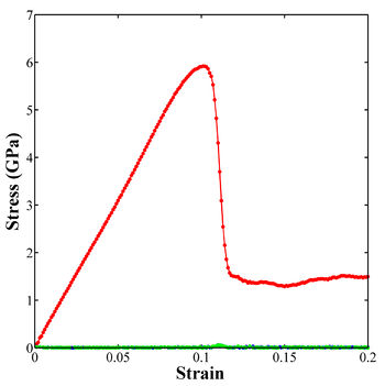
Figure 1. Stress-strain curve for uniaxial compressive loading of single crystal aluminum in the <100> loading direction.
Deformation Movie
This assumes that you already have AtomEye and ImageJ downloaded.- Visualize the dumpfile in AtomEye by typing the following command, "/A dump.tensile_0.cfg" (UNIX).
- Use the AtomEye options to select how you want to visualize deformation. In this example, the centrosymmetry parameter was used to show only atoms in a non-centrosymmetric environment (see Fig. 2).
- Use Alt+0 to activate centrosymmetric (csym) view.
- Adjust threshold, or set of atoms to view, by using Shift+T. This will allow creation of a set for the current parameter (in this case, csym). Please note that you need to adjust both lower and higher thresholds unless the atoms from following images that exceeds maximum value for the first one will be not shown. You can make it 5 or 10.
- Make atoms with values outside of the threshold invisible by using Ctrl+A.
- Press 'y' within AtomEye to produce an animation script.
- The folder "Jpg" now contains snapshots of all dumpfiles.
- Open ImageJ
- Drag the folder Jpg into ImageJ
- Select "Convert to RGB" to keep the color from the AtomEye images.
- Choose "yes" to load a stack.
- Adjust the size as needed (Image/Adjust/Size)
- Adjust frame rate as desired (Image/Stacks/Animation Options)
- Save as Animated Gif file
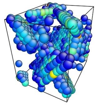
Figure 2. Image of nucleated dislocation near peak stress.
Movie showing compressive deformation of single crystal aluminum loaded in the <100> direction at a strain rate of 1010 s-1 and a temperature of 300 K. Only atoms in non-centrosymmetric environment are shown.
Deformation Movie using OVITO
In order for LAMMPS to output compatible data, one must set up an appropriate dump file with the desired data in the LAMMPS input script. Near the end of the LAMMPS script, use the 'dump' command in order to output desired data to a 'custom' file type for use in Ovito. The following lines create a dumpfile for every atom in the simulation every 250 timesteps, and each file is named according to its associated timestep. Then, the file is specified to show, for each atom, the atom ID, atom type, scaled atom coordinates, previously computed centrosymmetry and potential energy variables, and forces upon each atom.
# Dump to cfg for Ovito post processing
dump     1 all custom 250 dump.comp.* id type xs ys zs c_csym c_peratom fx fy fz
Now to make a movie using OVITO:
- Open Ovito.
- Select "File/Import," one of the dumpfiles you wish to animate, and "Open."
- Select "Use following wild-card name to load multiple files."
- You must tell Ovito what each column of data in the dumpfile is. Often, Ovito can do this for you if you click "Auto-assign columns."
- Use the Modifier List to add the desired modifications to your images and future animation. For this example, the "Common Neighbor Analysis" modifier was used to visualize dislocations.
- Test the animation by using the animation tools below the graphics.
- Click the "Render" tab.
- Select "Complete animation" and choose an output filename in "Output Filename." Save to a new directory for use later in ImageJ. Be sure to include an appropriate extension, such as ".bmp."
- Select the view that you would like to animate and click "Render Active Viewport" above "Render settings."
- Now you should have an image for every frame of your simulation.
Cell Size Comparison
In order to test the difference that the number of atoms can have on a simulation, the above script was run with 32,000 and 108,000 atoms in addition 4,000 atoms. Editing the values (currently "10") in the following line in the input script will change the size of the simulation cell and the number of atoms used in the simulation. Values of "20" will result in 32,000 atoms, and values of "30" will result in 108,000 atoms.
region whole block 0 10 0 10 0 10
Shown below are movies of the 4,000, 32,000, and 108,000 atom simulations, which show only atoms in a non-centrosymmetric environment. As one might expect, more slip planes become visible as the atom count of the simulation increases.
Movie showing compressive deformation of a 4,000 atom single crystal of aluminum loaded in the <100> direction. Only atoms in non-centrosymmetric environment are shown.
Movie showing compressive deformation of a 32,000 atom single crystal of aluminum loaded in the <100> direction. Only atoms in non- centrosymmetric environment are shown.
Movie showing compressive deformation of a 108,000 atom single crystal of aluminum loaded in the <100> direction. Only atoms in non-centrosymmetric environment are shown.
Temperature Comparison
The temperature of the simulations also makes a difference in the outputs. To show this difference, the above simulations (previously at 300 K) were run at 10 K. In order to change the temperature of the simulation, three lines in the input script must be edited. Two lie under the 'Equilibraion' section while the third lies under 'Deformation.'
The velocity and fix commands shown below contain temperature data. The velocity command specifies the thermal velocity of the system while the fix command specifies the desired temperatures at the beginning and end of the simulation. In order to run the simulation at 10 K instead of 300 K, change the three '300' values to '10' in the velocity and fix command lines.
# EQUILIBRATION
reset_timestep	0
timestep 0.001
velocity all create 300 12345 mom yes rot no
fix 1 all npt temp 300 300 1 iso 0 0 1 drag 1
The temperature values in the fix command under 'Deformation' also needs to be changed to '10' instead of '300.' The values are being changed again because between 'Equilibration' and 'Deformation' the fix ID 1 was unfixed. Here fix 1 is being redefined.
# DEFORMATION
reset_timestep	0

fix		1 all npt temp 300 300 1 y 0 0 1 z 0 0 1 drag 1
All three simulation cell sizes were run at 10 K. Below are the movies from the simulations. Once again, only atoms in a non-centrosymmetric environment are viewable. The difference between the 300 K and 10 K simulations is that there is less non-centrosymmetry induced by thermal velocity. At 10 K, many fewer atoms are seen before slip occurs, and the slip planes are more cleary visible and absent of "noise" created by atoms that are non-centrosymmetric solely due to thermal activity.
Movie showing compressive deformation of a 4,000 atom single crystal of aluminum at 10 K loaded in the <100> direction. Only atoms in non-centrosymmetric environment are shown.
Movie showing compressive deformation of a 32,000 atom single crystal of aluminum at 10 K loaded in the <100> direction. Only atoms in non-centrosymmetric environment are shown.
Movie showing compressive deformation of a 108,000 atom single crystal of aluminum at 10 Kloaded in the <100> direction. Only atoms in non-centrosymmetric environment are shown.
Questions and Answers?
Q1: I noticed that on the stress-strain curve in the Figure 1, following the peak stress (dislocation nucleation), the stresses are approximately 2 GPa in the strain range 0.1-0.2. However, in the log file and output files for the input script above, the stresses range from 2-6 GPa. Why?
A1: Aha! We threw a curveball at you. The plot is actually for a much larger simulation cell. The 4000-atom simulation cell from the above input script is relatively small. Hence, after dislocation nucleation, further plastic deformation becomes very difficult and you will actually see a second curve. For much larger cell sizes (and more atoms), this flow stress following nucleation should begin to look more like the stress-strain curve in Figure 1. This observation also brings up an important point - the behavior and properties calculated using molecular dynamics can sometimes be heavily influenced by the size of the simulation cell (and the strain rate and the potential and the temperature and the boundary conditions). I relate this size dependence in MD simulations to a mesh sensitivity study in finite element models - you should keep increasing the simulation cell size to understand the potential error in your calculations. If you can obtain some degree of convergence in properties or behavior (mechanism), this is the ideal situation.
Acknowledgments
The authors would like to acknowledge funding for this work through the Department of Energy.
References
- ↑ S. Plimpton, "Fast Parallel Algorithms for Short-Range Molecular Dynamics," J. Comp. Phys., 117, 1-19 (1995).
- ↑ Spearot, D.E., Tschopp, M.A., Jacob, K.I., McDowell, D.L., "Tensile strength of <100> and <110> tilt bicrystal copper interfaces," Acta Materialia 55 (2007) p. 705-714 (http://dx.doi.org/10.1016/j.actamat.2006.08.060).
- ↑ Tschopp, M.A., Spearot, D.E., McDowell, D.L., "Atomistic simulations of homogeneous dislocation nucleation in single crystal copper," Modelling and Simulation in Materials Science and Engineering 15 (2007) 693-709 ( http://dx.doi.org/10.1088/0965-0393/15/7/001).
- ↑ Tschopp, M.A., McDowell, D.L., "Influence of single crystal orientation on homogeneous dislocation nucleation under uniaxial loading," Journal of Mechanics and Physics of Solids 56 (2008) 1806-1830. (http://dx.doi.org/10.1016/j.jmps.2007.11.012).
- ↑ Y. Mishin, D. Farkas, M.J. Mehl, and D.A. Papaconstantopoulos, "Interatomic potentials for monoatomic metals from experimental data and ab initio calculations," Phys. Rev. B 59, 3393 (1999).
- ↑ J. Li, "AtomEye: an efficient atomistic configuration viewer," Modelling Simul. Mater. Sci. Eng. 11 (2003) 173.