
Integrated Computational Materials Engineering (ICME)
Uniaxial Tension
Abstract
This example script shows how to run an atomistic simulation of uniaxial tensile loading of an aluminum single crystal oriented in the <100> direction. This example uses a parallel molecular dynamics code, LAMMPS[1]. These scripts were initially used to study dislocation nucleation in single crystal aluminum and copper[2][3][4].
Author(s): Mark A. Tschopp, mtschopp@cavs.msstate.edu
Input
Description of Simulation
This molecular dynamics simulation first generates a simulation cell with fcc atoms with <100> orientations in the x, y, and z-directions. For this example, the simulation cell size is 10 lattice units in each direction, i.e., 4000 total atoms. Larger simulation cell sizes should be used to converge the dislocation nucleation stress values and to not influence the dislocation nucleation mechanism. The potential used here is the Mishin et al. (1999) aluminum potential[5]. The equilibration step allows the lattice to expand to a temperature of 300 K with a pressure of 0 bar at each simulation cell boundary. Then, the simulation cell is deformed in the x-direction at a strain rate of 1010 1/s, while the lateral boundaries are controlled using the NPT equations of motion to zero pressure. The stress and strain values are output to a separate file, which can be imported in a graphing application for plotting. The cfg dump files include the x, y, and z coordinates, the centrosymmetry values, the potential energies, and forces for each atom. This can be directly visualized using AtomEye[6].
Tensile Loading of an Aluminum Single Crystal. Movie showing deformation of single crystal aluminum loaded in the <100> direction at a strain rate of 1010 s-1 and a temperature of 300 K.
LAMMPS input script
This input script was run using the Aug 2015 version of LAMMPS. Changes in some commands in more recent versions may require revision of the input script. To run this script, store it in "in.tensile.txt" and then use "lmp_exe < in.tensile.txt" in a UNIX environment where "lmp_exe" refers to the LAMMPS executable.
# Input file for uniaxial tensile loading of single crystal aluminum
# Mark Tschopp, November 2010

# ------------------------ INITIALIZATION ----------------------------
units 		metal
dimension	3
boundary	p	p	p
atom_style	atomic
variable latparam equal 4.05

# ----------------------- ATOM DEFINITION ----------------------------
lattice		fcc ${latparam}
region		whole block 0 10 0 10 0 10
create_box	1 whole
lattice 	fcc ${latparam} orient x 1 0 0 orient y 0 1 0 orient z 0 0 1
create_atoms	1 region whole

# ------------------------ FORCE FIELDS ------------------------------
pair_style	eam/alloy
pair_coeff	* * Al99.eam.alloy Al

# ------------------------- SETTINGS ---------------------------------
compute csym all centro/atom fcc
compute peratom all pe/atom

######################################
# EQUILIBRATION
reset_timestep	0
timestep 0.001
velocity all create 300 12345 mom yes rot no
fix 1 all npt temp 300 300 1 iso 0 0 1 drag 1

# Set thermo output
thermo 1000
thermo_style custom step lx ly lz press pxx pyy pzz pe temp

# Run for at least 10 picosecond (assuming 1 fs timestep)
run 20000
unfix 1

# Store final cell length for strain calculations
variable tmp equal "lx"
variable L0 equal ${tmp}
print "Initial Length, L0: ${L0}"

######################################
# DEFORMATION
reset_timestep	0

fix		1 all npt temp 300 300 1 y 0 0 1 z 0 0 1 drag 1
variable srate equal 1.0e10
variable srate1 equal "v_srate / 1.0e12"
fix		2 all deform 1 x erate ${srate1} units box remap x

# Output strain and stress info to file
# for units metal, pressure is in [bars] = 100 [kPa] = 1/10000 [GPa]
# p2, p3, p4 are in GPa
variable strain equal "(lx - v_L0)/v_L0"
variable p1 equal "v_strain"
variable p2 equal "-pxx/10000"
variable p3 equal "-pyy/10000"
variable p4 equal "-pzz/10000"
fix def1 all print 100 "${p1} ${p2} ${p3} ${p4}" file Al_SC_100.def1.txt screen no

# Use cfg for AtomEye
dump 		1 all cfg 250 dump.tensile_*.cfg mass type xs ys zs c_csym c_peratom fx fy fz
dump_modify 1 element Al

# Display thermo
thermo 	1000
thermo_style	custom step v_strain temp v_p2 v_p3 v_p4 ke pe press

run		20000

######################################
# SIMULATION DONE
print "All done"
Output
LAMMPS logfile
The log.lammps file should look like this below. Notice that the 20 ps (20,000 fs) equilibration step brought the temperature of the simulation cell up to 300 K. The corresponding deformation went up to a strain of 0.2. The thermo command was set for every 1000 timesteps, so any plots should be made from the data included in the datafile.
LAMMPS (5 Nov 2010)
# Input file for uniaxial tensile loading of single crystal aluminum
# Mark Tschopp, November 2010

# ------------------------ INITIALIZATION ----------------------------
units 		metal
dimension	3
boundary	p	p	p
atom_style	atomic
variable latparam equal 4.05

# ----------------------- ATOM DEFINITION ----------------------------
lattice		fcc ${latparam}
lattice		fcc 4.05
Lattice spacing in x,y,z = 4.05 4.05 4.05
region		whole block 0 10 0 10 0 10
create_box	1 whole
Created orthogonal box = (0 0 0) to (40.5 40.5 40.5)
  2 by 2 by 2 processor grid

region		upper block INF INF INF INF INF INF units box
lattice 	fcc ${latparam} orient x 1 0 0 orient y 0 1 0 orient z 0 0 1
lattice 	fcc 4.05 orient x 1 0 0 orient y 0 1 0 orient z 0 0 1
Lattice spacing in x,y,z = 4.05 4.05 4.05
create_atoms	1 region upper
Created 4000 atoms

# ------------------------ FORCE FIELDS ------------------------------
pair_style	eam/alloy
pair_coeff	* * Al99.eam.alloy Al

# ------------------------- SETTINGS ---------------------------------
compute csym all centro/atom fcc
compute peratom all pe/atom

######################################
# EQUILIBRATION
reset_timestep	0
timestep 0.001
velocity all create 300 12345 mom yes rot no
fix 1 all npt temp 300 300 1 iso 0 0 1 drag 1

# Set thermo output
thermo 1000
thermo_style custom step lx ly lz press pxx pyy pzz pe temp

# Run for at least 10 picosecond (assuming 1 fs timestep)
run 20000
Memory usage per processor = 2.55571 Mbytes
Step Lx Ly Lz Press Pxx Pyy Pzz PotEng Temp
       0         40.5         40.5         40.5    2496.1233    2446.9902    2534.6541    2506.7256       -13440          300
    1000    40.558342    40.558342    40.558342    731.50829    755.55351    696.37101    742.60035   -13363.301    169.49172
    2000    40.574199    40.574199    40.574199    106.78935   -46.253007    296.26883    70.352219   -13356.097    178.17311
    3000    40.579471    40.579471    40.579471    314.81803    314.71612    292.22553    337.51245   -13347.025      183.623
    4000    40.586697    40.586697    40.586697    107.84524    52.829414    112.73441     157.9719   -13340.823    194.61149
    5000    40.593224    40.593224    40.593224    172.67874    158.86784    199.13978    160.02861   -13334.364    204.85854
    6000    40.601567    40.601567    40.601567    56.953653   -6.2830484   -16.301111    193.44512    -13327.55    213.93605
    7000     40.60782     40.60782     40.60782    31.891969    35.437938    63.396951   -3.1589825    -13320.86    222.48071
    8000    40.616908    40.616908    40.616908   -244.41321   -212.11716   -305.70692   -215.41555   -13317.384      236.254
    9000    40.618876    40.618876    40.618876    13.561356    111.07353   -29.999797   -40.389663   -13313.071    247.18002
   10000    40.625506    40.625506    40.625506   -125.06329    -105.4566   -93.514599   -176.21866   -13308.875    256.93613
   11000    40.631525    40.631525    40.631525   -75.690987    141.36136    14.068057   -382.50238   -13303.582    263.00631
   12000    40.631815    40.631815    40.631815     79.38005    63.796397    144.76416    29.579595    -13299.23    269.23326
   13000    40.637408    40.637408    40.637408    -152.9113   -399.37081   -31.484802   -27.878283   -13298.162     280.0582
   14000    40.636962    40.636962    40.636962    237.09239    58.799334    196.78768    455.69014   -13294.166    283.43969
   15000    40.641455    40.641455    40.641455    105.44503    114.55343     142.4659    59.315739   -13291.527    287.73561
   16000    40.643072    40.643072    40.643072    82.986611   -130.36308     288.9926    90.330318   -13288.384    289.39655
   17000     40.64789     40.64789     40.64789   -12.310673   -112.67891    -132.8659     208.6128   -13289.081    296.89271
   18000    40.644319    40.644319    40.644319    269.36896    180.82571    218.97472    408.30644   -13286.862    297.25615
   19000    40.646772    40.646772    40.646772    166.57104    20.881491   -79.807885    558.63952   -13287.577    301.80321
   20000    40.649126    40.649126    40.649126    116.57534   -108.86953    156.54682    302.04873   -13284.646    298.01867
Loop time of 81.5242 on 8 procs for 20000 steps with 4000 atoms

Pair  time (%) = 64.1903 (78.7378)
Neigh time (%) = 0 (0)
Comm  time (%) = 13.9448 (17.1051)
Outpt time (%) = 0.00286543 (0.00351483)
Other time (%) = 3.38623 (4.15365)

Nlocal:    500 ave 500 max 500 min
Histogram: 8 0 0 0 0 0 0 0 0 0
Nghost:    2930 ave 2930 max 2930 min
Histogram: 8 0 0 0 0 0 0 0 0 0
Neighs:    35000 ave 36430 max 33540 min
Histogram: 2 0 1 1 0 0 1 1 0 2
FullNghs: 0 ave 0 max 0 min
Histogram: 8 0 0 0 0 0 0 0 0 0

Total # of neighbors = 280000
Ave neighs/atom = 70
Neighbor list builds = 0
Dangerous builds = 0
unfix 1

# Store final cell length for strain calculations
variable tmp equal "lx"
variable L0 equal ${tmp}
variable L0 equal 40.64912642
print "Initial Length, L0: ${L0}"
Initial Length, L0: 40.64912642

######################################
# DEFORMATION
reset_timestep	0

fix		1 all npt temp 300 300 1 y 0 0 1 z 0 0 1 drag 1
variable srate equal 1.0e10
variable srate1 equal "v_srate / 1.0e12"
fix		2 all deform 1 x erate ${srate1} units box remap x
fix		2 all deform 1 x erate 0.01 units box remap x

# Output strain and stress info to file
# for units metal, pressure is in [bars] = 100 [kPa] = 1/10000 [GPa]
# p2, p3, p4 are in GPa
variable strain equal "(lx - v_L0)/v_L0"
variable p1 equal "v_strain"
variable p2 equal "-pxx/10000"
variable p3 equal "-pyy/10000"
variable p4 equal "-pzz/10000"
fix def1 all print 100 "${p1} ${p2} ${p3} ${p4}" file Al_SC_100.def1.txt screen no

# Use cfg for AtomEye
dump 		1 all cfg 250 dump.tensile_*.cfg id type xs ys zs c_csym c_peratom fx fy fz
dump_modify 1 element Al

# Display thermo
thermo 	1000
thermo_style	custom step v_strain temp v_p2 v_p3 v_p4 ke pe press

run		20000
Memory usage per processor = 2.8622 Mbytes
Step strain Temp p2 p3 p4 KinEng PotEng Press
       0 -8.7965858e-11    298.01867  0.010886953 -0.015654682 -0.030204873    154.04923   -13284.646    116.57534
    1000 0.0099999999    301.40099   0.67990399  0.067064258 0.0053203864    155.79758   -13283.836   -2507.6288
    2000         0.02    298.01046    1.2830198  0.019592784 -0.036714858    154.04498   -13276.743   -4219.6592
    3000         0.03    304.39575    1.9202839  0.064889677  0.016160978    157.34561    -13271.94    -6671.115
    4000         0.04    293.49046    2.5079447 -0.011621532 -0.045248722    151.70854   -13255.553   -8170.2481
    5000         0.05    299.61448    3.1080399 -0.0063053351 -0.001951119    154.87412   -13245.404   -10332.611
    6000         0.06    301.13685    3.7262713 -0.018319706  0.058027821    155.66105    -13230.48   -12553.265
    7000         0.07    304.50008    4.3068752  0.036084841  0.022188973    157.39954    -13214.12   -14550.497
    8000         0.08    301.24768    4.8543157 -0.0043461496 0.0099095843    155.71833   -13192.071   -16199.597
    9000         0.09    295.90445    5.3741975 -0.0084256638 -0.013966722    152.95636   -13166.694    -17839.35
   10000          0.1    292.31188    5.8552584 -0.023696478 -0.020282681    151.09932   -13139.944   -19370.931
   11000         0.11    298.84284    6.4501419  0.017547204  0.015913195    154.47525    -13116.23   -21612.008
   12000         0.12     295.8812     6.918376 -0.027979731  0.033011555    152.94434   -13085.401   -23078.026
   13000         0.13     296.6501    7.4105164  0.040017275  0.063746831     153.3418   -13054.406   -25047.602
   14000         0.14    291.84214    7.7838516  0.010140057 -0.050282654    150.85651   -13018.661   -25812.363
   15000         0.15    290.68698    7.9945223   0.04870559  0.076553482    150.25939   -12983.262   -27065.938
   16000         0.16    377.39464    2.6003776  0.022766694 0.0045660696    195.07956   -13008.794   -8759.0346
   17000         0.17    412.37758    1.2494147 -0.0087695036  0.018247454    213.16264   -13041.345   -4196.3088
   18000         0.18    429.78685   0.95088514 -0.078803047  0.051915067    222.16169   -13073.821   -3079.9905
   19000         0.19    427.62458   0.98387526  0.017524712  0.053337669    221.04399   -13096.987   -3515.7922
   20000          0.2    410.07663    1.1025637  0.010470766 -0.082932084    211.97325   -13109.962   -3433.6746
Loop time of 96.4415 on 8 procs for 20000 steps with 4000 atoms

Pair  time (%) = 74.4147 (77.1605)
Neigh time (%) = 0.131499 (0.136351)
Comm  time (%) = 13.7462 (14.2534)
Outpt time (%) = 2.21778 (2.29961)
Other time (%) = 5.93133 (6.15019)

Nlocal:    500 ave 517 max 489 min
Histogram: 1 2 0 1 1 2 0 0 0 1
Nghost:    2457.88 ave 2466 max 2437 min
Histogram: 1 0 0 0 0 1 1 1 1 3
Neighs:    34511 ave 35305 max 33225 min
Histogram: 1 1 0 1 0 0 0 1 0 4
FullNghs: 69094.8 ave 71637 max 67679 min
Histogram: 2 1 0 1 2 1 0 0 0 1

Total # of neighbors = 552758
Ave neighs/atom = 138.19
Neighbor list builds = 67
Dangerous builds = 0

######################################
# SIMULATION DONE
print "All done"
All done
LAMMPS datafile
The following datafile was also generated during this simulation.
# Fix print output for fix def1
0.0009999999119 0.08667300618 0.03175758225 0.03801213452
0.001999999912 0.09131420312 -0.05499624531 -0.03396621651
0.002999999912 0.2254889267 0.04825004506 0.04680554658
0.003999999912 0.2199842183 -0.04156649661 -0.02074145126
0.004999999912 0.3127067321 0.01435171918 0.01093418588
...
LAMMPS dumpfile
The following dumpfile in cfg format was also generated during this simulation.
Number of particles = 4000
A = 1.0 Angstrom (basic length-scale)
H0(1,1) = 40.6491 A
H0(1,2) = 0 A
H0(1,3) = 0 A
H0(2,1) = 0 A
H0(2,2) = 40.6491 A
H0(2,3) = 0 A
H0(3,1) = 0 A
H0(3,2) = 0 A
H0(3,3) = 40.6491 A
.NO_VELOCITY.
entry_count = 8
auxiliary[0] = csym
auxiliary[1] = peratom
auxiliary[2] = fx
auxiliary[3] = fy
auxiliary[4] = fz
26.982
Al
0.0493442 0.0581882 0.00323696 1.58804 -3.34266 0.196691 -0.804728 -0.0280286
0.0987502 0.00417997 0.00238952 0.827133 -3.34273 -0.475844 -0.270217 -0.120716
0.0989802 0.0523976 0.0521907 0.363772 -3.30304 -0.309005 -0.274515 -0.299433
0.0495058 0.102418 0.0536544 0.611128 -3.30518 0.162097 -0.42069 -0.15808
0.0995051 0.102793 0.00119416 0.614289 -3.28181 -0.406727 -0.192102 0.405813
0.0473774 0.0488825 0.10204 0.581043 -3.3709 0.135458 -0.205472 -0.294232
0.0989535 0.000697083 0.0977144 0.583569 -3.30702 -0.474259 0.0845695 0.400838
...
POST-PROCESSING
Stress-Strain Plot
The stress-strain curve in Figure 1 can be generated using the following MATLAB script:
%% Analyze def1.txt files
% Plot the various responses

d = dir('*.def1.txt');
for i = 1:length(d)
    % Get data
    fname = d(i).name;
    A = importdata(fname);
    strain = A.data(:,1);
    stress = A.data(:,2:4);

    % Generate plot
    plot(strain,stress(:,1),'-or','LineWidth',2,'MarkerEdgeColor','r',...
                'MarkerFaceColor','r','MarkerSize',5),hold on
    plot(strain,stress(:,2),'-ob','LineWidth',2,'MarkerEdgeColor','b',...
                'MarkerFaceColor','b','MarkerSize',5),hold on
    plot(strain,stress(:,3),'-og','LineWidth',2,'MarkerEdgeColor','g',...
                'MarkerFaceColor','g','MarkerSize',5),hold on
    axis square
    ylim([0 10])
    set(gca,'LineWidth',2,'FontSize',24,'FontWeight','normal','FontName','Times')
    set(get(gca,'XLabel'),'String','Strain','FontSize',32,'FontWeight','bold','FontName','Times')
    set(get(gca,'YLabel'),'String','Stress (GPa)','FontSize',32,'FontWeight','bold','FontName','Times')
    set(gcf,'Position',[1 1 round(1000) round(1000)])

    % Export figure to tif file
    exportfig(gcf,strrep(fname,'.def1.txt','.tif'),'Format','tiff',...
    'Color','rgb','Resolution',300)
    close(1)

    end
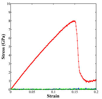
Figure 1. Stress-strain curve for uniaxial tensile loading of single crystal aluminum in the <100> loading direction.
The exportfig command refers to a script on MATLAB Central File website. You will need to go to the website and download the script into the current directory for this to work.
Deformation Movie
First download AtomEye.- Go to AtomEye website.
- Download the A.i686 version by right-clicking on the link and "Save Target As..." to one of your directories.
- Rename the downloaded file as A by typing "cp A.i686 A". A will be the executable.
- Using UNIX, run "chmod A 755" on the file to change this to an executable.
- To test, you need to save a CFG file as well, such as cnt8x3.cfg. Try running using "./A cnt8x3.cfg".
- Go to ImageJ website.
- Download the appropriate version for Windows, LINUX, or MAC.
- Visualize the dumpfile in AtomEye by typing the following command, "/A dump.tensile_0.cfg" (UNIX).
- Use the AtomEye options to select how you want to visualize deformation. In this example, the centrosymmetry parameter was used to show only atoms in a non-centrosymmetric environment (see Fig. 2).
- Use Alt+0 to activate centrosymmetric (csym) view.
- Adjust threshold, or set of atoms to view, by using Shift+T. This will allow creation of a set for the current parameter (in this case, csym). Please note that you need to adjust both lower and higher thresholds unless the atoms from following images that exceeds maximum value for the first one will be not shown. You can make it 5 or 10.
- Make atoms with values outside of the threshold invisible by using Ctrl+A.
- Press 'y' within AtomEye to produce an animation script.
- The folder "Jpg" now contains snapshots of all dumpfiles.
- Open ImageJ
- Drag the folder Jpg into ImageJ
- Select "Convert to RGB" to keep the color from the AtomEye images.
- Choose "yes" to load a stack.
- Adjust the size as needed (Image/Adjust/Size)
- Adjust frame rate as desired (Image/Stacks/Tools/Animation Options)
- Save as Animated Gif file
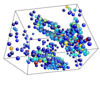
Figure 2. Image of nucleated dislocation near peak stress.
Tensile Loading of an Aluminum Single Crystal. Movie showing deformation of single crystal aluminum loaded in the <100> direction at a strain rate of 1010 s-1 and a temperature of 300 K. Only atoms in non-centrosymmetric environment are shown.
Questions and Answers?
Q1: I ran this tutorial of an atomistic simulation of uniaxial tensile loading of an aluminum single crystal oriented in the <100> direction. However, I want to use the LJ potential instead of the EAM potential. When I run the input script with the Lennard Jones potential, I get much different results. The stress is nearly 3 times the stress from the EAM potential. I don't know where something is wrong.
A1: Interatomic potentials play a commanding role in the properties of molecular dynamics simulations. The most simple potential is the Lennard Jones potential. The embedded atom method potential is a little more sophisticated and I would encourage you to look up the original papers by Mike Baskes (1983, 1984) to examine how this common potential formulation was created. While there are an increasing number of potential formulations out there now and an increasing number of potentials, the embedded atom method has been widely used over the years and still is. However, this brings up the point that different potentials may give vastly different properties because each potential may have been formulated for a particular problem. It is up to the user to decide whether the potential seems to give plausible results for their application or whether the initial fitting contains properties that are important for their application.
Acknowledgements
The authors would like to acknowledge funding for this work through the Department of Energy.
References
- ↑ S. Plimpton, "Fast Parallel Algorithms for Short-Range Molecular Dynamics," J. Comp. Phys., 117, 1-19 (1995).
- ↑ Spearot, D.E., Tschopp, M.A., Jacob, K.I., McDowell, D.L., "Tensile strength of <100> and <110> tilt bicrystal copper interfaces," Acta Materialia 55 (2007) p. 705-714 (http://dx.doi.org/10.1016/j.actamat.2006.08.060).
- ↑ Tschopp, M.A., Spearot, D.E., McDowell, D.L., "Atomistic simulations of homogeneous dislocation nucleation in single crystal copper," Modelling and Simulation in Materials Science and Engineering 15 (2007) 693-709 (http://dx.doi.org/10.1088/0965-0393/15/7/001).
- ↑ Tschopp, M.A., McDowell, D.L., "Influence of single crystal orientation on homogeneous dislocation nucleation under uniaxial loading," Journal of Mechanics and Physics of Solids 56 (2008) 1806-1830. (http://dx.doi.org/10.1016/j.jmps.2007.11.012).
- ↑ Y. Mishin, D. Farkas, M.J. Mehl, and D.A. Papaconstantopoulos, "Interatomic potentials for monoatomic metals from experimental data and ab initio calculations," Phys. Rev. B 59, 3393 (1999).
- ↑ J. Li, "AtomEye: an efficient atomistic configuration viewer," Modelling Simul. Mater. Sci. Eng. 11 (2003) 173.