Integrated Computational Materials Engineering (ICME)
Uncertainty
Overview

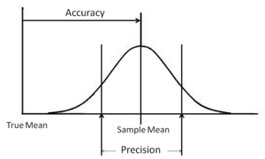
Fig 1. Random (precision) and Bias (accuracy) Uncertainty related to a distribution of measurements.

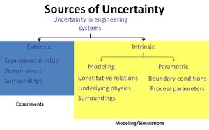
Fig 2. Intrinsic (internal) and Extrinsic (external) Uncertainty sources for engineering systems from the modeling point of view.
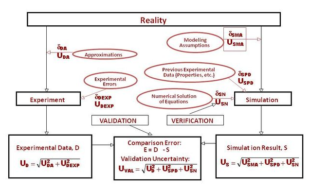
Uncertainty Quantification (UQ) is the science of quantitative characterization and reduction of uncertainties in applications. The purpose of UQ is to determine the most likely outcome from models where inputs are not exactly known and help designers to determine the confidence in modeling predictions. In this way, UQ is inherently tied to the concept of Verification and Validation (V&V) of modeling frameworks, and therefore very important within the context of Integrated Computational Materials Engineering (ICME).
Here Verification is defined as the process of determining that a model implementation accurately represents the developer's conceptual description of the model (i.e. "doing things right"). Validation is defined as the process of determining the degree to which a model is an accurate representation of the real world for the intended uses of the model (i.e. "doing the right thing").
Qualitatively, uncertainty is the possibility of error in measurement and modeling of physical phenomenon. Uncertainty, in the context of engineering, is the quantification of the possible distribution of errors in measurements of an experiment. These measurements, when used for modeling, can effect the accuracy and precision of calculations. In the context of modeling, the most common methodology to account for the inaccuracy and imprecision of measured parameters is the use of Monte Carlo (MC) simulation techniques. In these methods, representative statistical distributions for each model parameter are randomly sampled to generate thousands of simulation points which are then mapped to model outputs. Descriptive statistics are then calculated for the modeling output.
In Uncertainty Quantification (UQ) there are many sources of uncertainty for engineering systems. From the modeling frame of reference, these uncertainties can come from modeling assumptions and simplifications (intrinsic) or from model calibrations using uncertain data (extrinsic). These extrinsic uncertainties can arise from measurement system errors (e.g. bad calibrations) and simplifications of experimental boundary conditions. Figure 1 details the sources of uncertainty for engineering systems. These uncertainties generally fall into two categories: bias (systematic) and random (repeatability) uncertainty.
Random (repeatability) uncertainty derives from natural variation in repeated measurements and is directly linked to the precision of a measurment system. The more precise the measurement system, the "slimmer" the distribution.
Bias (systematic) uncertainty derives from the use of a measurement system and can be introduced due to human faults such as bad measurement system calibration or inconsistent measurement system use. This type of uncertainty can be harder to quantify since not every technician will use a measurement system the same. To minimize this type of error, it is good practice to create a standard operating procedure (SOP) so that errors will be uniform across all users as well as calibrating the measurement system to a "gold standard". The more accurate (less biased) the measurement system, the closer a sample mean of a set of measurements will be to the true value.
Performed in conjunction, a sensitivity analysis seeks to describe the sensitivity (in other words, the expected variability) of model output with respect to variability in model parameters. It allows for the ranking of modeling parameters in order of their effect on the modeling output. There are various techniques used to rank parameters according to their sensitivity measure which fall into two major categories: local methods and global methods.
Local sensitivities seek to describe the expected change in model output around a fixed point in the model's input space; hence the term local since the range of relevance is only around this fixed model input point in N-dimensional space. Generally, perturbation methods are used to evaluate the local derivatives by approximation using forward finite differences, backward finite differences, or central finite differences. If the equations are well-behaved (not highly nonlinear, closed-form, and continuous) and not overly complex, analytical partial derivatives can be obtained by differentiation and solved directly. Local sensitivity analyses are generally used in the model calibration stage to give an idea of calibration precision and accuracy. This type of sensitivity measure can also aid in model calibration since it gives information about the effect of a specific variable at a specific point of the calibration curve.
Global sensitivities seek describe the overall effect of a parameter's input range on the entirety of the solution space. Effectively, this method seeks to determine the average effect of the parameter by utilizing the entirety of the input range; that is, the model is not confined to a single N-dimensional model point, but the entirety of the input range is inspected for each variable in the model. There are various measures for global sensitivity, namely First Order Effect Index and Total Effect Index. First order indices only measure the contribution of a single variable on model output variance and do not describe any possible interactions between variables. Total effect indices describe the total contribution to the total variance of a model including the possible interactions between variances (i.e. conditional variances), however these measures are typically more computationally expensive.
Tutorials
Methods
Quantifying Experimental Uncertainties
Confidence intervals are a general method used in quantifying the uncertainty of experimental measurements. Equation 1 shows the confidence interval associated with the normal (Gaussian) probability distribution. For many engineering applications, measurements are usually assumed to adhere to a normal distribution if data is sparse. However, if considerable data is available such that the actual probability distribution can be obtained, it is best to use a confidence interval for its specific distribution (Uniform, Normal, Log Normal, Weibull, Brinbaum-Saunders, Poisson, etc...).
Where  is an estimator from the sample standard normal distribution with degrees of freedom
  and significance level
  , and
, and  is the sample standard deviation of
  measurements.
For some complex distributions (Weibull, Birnbaum-Saunders) that contain constants that cannot be obtained from data analysis, Maximum Likelihood Estimation (MLE) routines must be employed to compute the distribution constants.
Analysis Methods
Propagation of Uncertainty
Often used for closed form, deterministic models, this methodology uses a mathematical treatment based in statistics to propagate the uncertainty of the measured variables (inputs) to the result (output) of a model. A common methodology called the General Uncertainty Analysis is a truncated Taylor series expansion method and is explained in depth by Coleman et al[1] and is represented by the following equation:
Where  is the sensitivity of the output function
  to the input
  and
and  is the component uncertainty associated with the input variable
  . Since the input uncertainty is a constant, the mathematics of the model can either magnify or reduce the contribution of uncertainty from an input. These methods take advantage of linear superposition principles for models that can be approximated with well-behaved Taylor series expansions. For models that display high nonlinearity where the magnitudes of the sensitivities are disperate, different Uncertainty Quantification (UQ) methods may be needed (e.g. Monte Carlo, Latin Hypercube...).
Statistical Methods
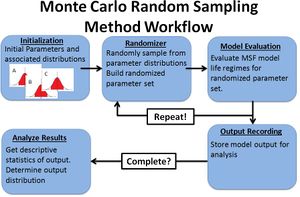
When the application of the propagation method is either too tedious (e.g very large model), impossible (e.g. not closed form), or inappropriate (e.g. highly nonlinear) a statistical method is necessary. The most common method for quantifying uncertainty in modeling subjected to uncertain inputs is the Monte Carlo (MC) method. This method involves sampling from a representative statistical distribution for each model parameter to generate thousands of model input points (e.g.  ). Generally a very high number of observations are simulated to adequately describe how the input parameters vary to describe the interactions of one variable on another as well as their effect on model output. Using the output data and descriptive statistics, the statistical distribution of the output can be determined with respect to the input distributions. Figure 3 shows the general workflow for a Monte Carlo Random Sampling scheme.

Fig 3. Monte Carlo Random Sampling Workflow example.
Analysis Tools
Sandia National Labs, Dakota
Sandia National Labs maintains an extensive, general purpose analysis tool for the purpose of optimization, sensitivity analysis, and uncertainty quantification. More information can be found on their website at: https://dakota.sandia.gov/
Uncertainty Quantification and Sensitivity Analysis (UQSA) Tool
A simple, generalized forward propagation platform for uncertainty quantification (UQ) and sensitivity analysis (SA) is in development for experimental and modeling efforts. Version 1.3 is available for use at the following link:
Applications
Microstructure Sensitive MultiStage Fatigue (MSF) Model
Authors: J. D. Bernard, J.B. Jordan, M. Lugo, J.M. Hughes, D.C. Rayborn, M.F. Horstemeyer
Abstract[2]
DOI: https://dx.doi.org/10.1016/j.ijfatigue.2013.02.015
The objective of this paper is to quantify the microstructurally small fatigue crack growth of an extruded AZ61 magnesium alloy. Fully reversed and interrupted load-controlled tests were conducted on notched specimens that were taken from the material in the longitudinal and transverse orientations with respect to the extrusion direction.In order to measure crack growth,replicas of the notch surface were made using a dual-step silicon-rubber compound at periodic cyclic intervals.By using mic roscopic analysis of the replica surfaces, crack initiation sites from numer ous locations and crack growth rates were deter- mined. Amarked acceleration/deceleration was observed to occur in cracks of smaller length scales due to local microheterogeneities consistent with prior observ ations of small fatigue crack interaction with the native microstructure and texture. Finally,amicrostructure-sensitive multistage fatigue model was employed to estimate the observ ed crack growth behavior and fatigue life with respect to the microstruc- ture with the most notable item being the grain orientation.The crack growt hrate and fatigue life esti- mates are shown to compare well to published findingsfor pure magnesium single crystal atomistic simulations.
Microstructure Sensitive Internal State Variable (ISV) Modeling
Author(s): Kiran N. Solanki
Abstract

Understanding the effect of material microstructural heterogeneities and the associated mechanical property uncertainties in the design and the maintenance phases of engineering systems are pivotal not only in terms of successful development of reliable, safe, and economical systems but also for the development of a new generation of lightweight designs and predication capability[3][1]. Engineering systems contain different kinds of uncertainties found in material and component structures, computational models, input variables, and constraints[4][5]. Potential sources of uncertainty in a system include human errors, manufacturing or processing variations, operating condition variations, inaccurate or insufficient data, assumptions and idealizations, and lack of knowledge[3]. Since engineering materials are complex, hierarchical, and heterogeneous systems, adopting a deterministic approach to engineering designs may be limiting[6]. First, microstructure is inherently random at different scales. Second, parameters of a given model are subject to variations associated with variations of material microstructure from specimen to specimen[7]. Furthermore, uncertainty should be associated with model-based predictions for several reasons. Models inevitably incorporate assumptions and approximations that impact the precision and accuracy of predictions. Uncertainty may increase when a model is used near the limits of its intended domain of applicability and when information propagates through a series of models. Experimental data for conditioning or validating approximate (or detailed) models may be sparse and may be affected by measurement errors. Also, uncertainty can be associated with the structural member tolerance differences and morphologies of realized material microstructure due to variations in processing history. Often, it is expensive or impossible to remove and measure these sources of variability, but their impact on model predictions and final system performance can be profound.
Some of the formidable research challenges associated with the integration of advanced (multiscale) computational tools into a computational design framework include uncertainty quantification and the efficient coupling of such material models with nonlinear static and transient dynamic finite element analysis (FEA) of structures, as well as the development of non-deterministic approaches and solution strategies for design optimization under uncertainty[4]. At CAVS, we employ hierarchy of experimental data and material microstructure information to quantify uncertainties through calibration, validation, and verification in the context of materials design and its failure progression mechanisms[8].
Modified Embedded-Atom Method (MEAM)
Applications
- Structural Scale
- Macroscale
- Electronic Scale
- Hierarchical Bridging Between Ab Initio and Atomistic Level Computations: Calibrating the Modified Embedded Atom Method (MEAM) Potential (Part A)
- Hierarchical Bridging Between Ab Initio and Atomistic Level Computations: Sensitivity and Uncertainty Analysis for the Modified Embedded Atom Method (MEAM) Potential (Part B)
References
- ↑ Coleman, H.W., and Steele, G.W (2010) Experimentation and Uncertainty Analysis for Engineers.
- ↑ Bernard, J.D., Jordan, J.B., Lugo,M., Hughes, J.M., Rayborn, D.C., Horstemeyer, M.F., (2013), IJF (https://dx.doi.org/10.1016/j.ijfatigue.2013.02.015).
- ↑ Solanki, K.N., (2008), In Mississippi State University (Eds.), Ph.D. Dissertation(https://sun.library.msstate.edu/ETD-db/theses/available/etd-11062008-200935/).
- ↑ Solanki, K.N., Acar, E., Rais-Rohani, M., Horstemeyer, M., & Steele, G. (2009). IJDE 1(2) (https://www.inderscience.com/search/index.php?action=record&rec_id=28446/).
- ↑ https://catalog.asme.org/Codes/PrintBook/B89732_2007_Guidelines.cfm
- ↑ Solanki, K.N., Horstemeyer, M.F., Steele, G.W., Hammi, Y., & Jordon, J.B. (2009), IJSS(https://dx.doi.org/10.1016/j.ijsolstr.2009.09.025).
- ↑ Horstemeyer, M.F., Solanki, K.N., and Steele, W.G., (2005). In the proceeding of int. Plasticity Con.
- ↑ https://catalog.asme.org/Codes/PrintBook/VV_10_2006_Guide_Verification.cfm


