
Integrated Computational Materials Engineering (ICME)
Uncertainty Quantification and Sensitivity Analysis Tool
Introduction and Download
The Uncertainty Quantification and Sensitivity Analysis tool (UQSA), is a general platform for forward propagation analysis of various analytical engineering models. Written in the scripting language Python 2.7, this tool is a collection of scripts written by researchers at the Center for Advanced Vehicular Systems (CAVS) and published here for general use. Due to syntax differences between Python 2.7 and Python 3.5, these scripts will not run in Python 3.5. All code is subject to the MIT open-source license. By downloading these python scripts, you accept the conditions of the MIT open-source license. The license is available as a header for all contained scripts.- Download UQSA tool (Python) (Git repository)
- Current features:
- Monte Carlo random sampling for uncertainty propagation, capable of sampling from gaussian or uniform distributions
- General Uncertainty Analysis
- Local sensitivity measures (normalized and non-normalized local partial derivatives)
- Global Sensitivity measures
- First Order Effect Indices using Monte Carlo random sampling
- First Order Effect Indices using Fourier Amplitude Sensitivity Test (FAST) method using standard uniform distribution parameter search curves
- Radial Basis Function Network (RBFN) surrogate model
- Planned Features:
- Total Effect Indices using the Extended Fourier Amplitude Sensitivity Test (EFAST)
- Current features:
Environment Setup
Python Version
The Uncertainty Quantification and Sensitivity Analysis (UQSA) tool is written in the programming language Python and takes advantage of existing open-source packages. In order to use the Python version of this tool, the following external packages must be installed depending on your operating system.Windows
In Windows, Anaconda Python is the easiest Python build to install and update. Once installed, to update Python to the newest available version, open a command prompt and use the following command:conda update python
Linux
Most Linux distributions have Python pre-installed (Ubuntu/Debian/Redhat). If this is the case, skip to "Install Python Packages."Build and Install Python
Install required dependecies:
$ sudo apt-get install build-essential checkinstall
$ sudo apt-get install libreadline-gplv2-dev libncursesw5-dev
$ sudo apt-get install libssl-dev libsqlite3-dev tk-dev
$ sudo apt-get install libgdbm-dev libc6-dev libbz2-dev
Download and install Python 2.7
$ cd /usr/src
$ wget https://www.python.org/ftp/python/2.7.10/Python-2.7.11.tgz
$ tar xzf Python-2.7.11.tgz
$ cd Python-2.7.11
$ sudo ./configure
$ sudo make altinstall
Install Python Packages
Common Linux Installation The following is for basic Python functionality in Ubuntu/Debian versions of Linux, use the following commands in terminal to install the required packages. Anaconda Python users should use the existing "conda" package manager.
$ sudo apt-get install python-numpy python-scipy python-matplotlib
For Fedora/Redhat users, use the following commands in terminal to install the required packages.
$ sudo yum install numpy scipy python-matplotlib
Anaconda Python First, install Anaconda Python. Anaconda Python users can use the following commands to install the dependencies in a new Python environment. If you would like to install packages to thebase Python directory, skip to step 3.
#Step 1: Create new python environment
conda create --name py27

#Step 2: Activate new python environment
source activate py27 (Linux)
activate py27 (Windows)

#Step 3: Install Packages (ensure that your new environment is activated, otherwise this will install to the base python package)
conda update python
conda install numpy scipy matplotlib
Methodologies
Uncertainty Quantification
General Uncertainty Analysis
Often used for closed form, deterministic models, this methodology uses a mathematical treatment based in statistics to propagate the uncertainty of the measured variables (inputs) to the result (output) of a model. A common methodology, the General Uncertainty Analysis, is explained in depth by Coleman et al. [1] and is represented by the following equation: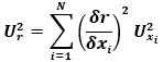
Where
Monte Carlo Random Sampling
When the application of the propagation method is inappropriate (e.g., highly nonlinear, disparate partial derivative magnitudes) a statistical method is necessary. The most common method for quantifying uncertainty in modeling subjected to uncertain inputs is the brute force Monte Carlo (MC) method. This method involves sampling from a representative statistical distribution for each model parameter to generate thousands of model input points (e.g., {x1,x2,…,xn }). Generally, a very high number of observations are simulated to adequately describe how the input parameters vary in combination with all other variables in the analysis. Using the output data and descriptive statistics, the statistical distribution of the output can be determined with respect to the input distributions. Figure 1 shows the general workflow for a Monte Carlo Random Sampling scheme.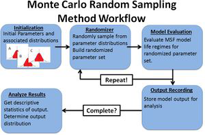
Fig 1. Monte Carlo Random Sampling Workflow example.
The UQSA tool uses a simple random sampling Monte Carlo routine. That means that sampling is not filtered or constrained in any way.
Sensitivity Analysis
Local Sensitivity Analysis
Local sensitivity analysis techniques employ the evaluation of partial derivative terms around an N-dimensional model calibration point. As such, these sensitivity measures are only applicable at the model point used, hence the term local. This method is best used in the model calibration stages of material model development as it allows for researchers to fine tune the parameters that have the greatest effect on model output and provide a basis for reducing calibration error. As stated, this measure is simply the raw numerical values of the partial derivatives of a model: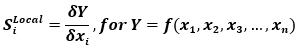
Where Y is the model of interest and the xi's are the model inputs. However, each sensitivity measure for each xi cannot be directly compared due to issues with units. If combined model parameter input and output standard deviations, the local derivatives can be normalized using the input and output standard deviations:
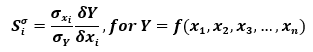
Where is the ith parameter standard deviation and σY is the standard deviation of the model output subjected to variation of all parameters. These measures are called "sigma normalized local sensitivities" and allow for the direct comparison between parameters and their expected contribution to the model output variance. When derivative information is selected to be output from the UQSA tool and a Monte Carlo analysis of uncertainty is performed, the input and output standard deviations from model simulations are used to normalize the partial derivative terms. Otherwise, just the raw numerical values of the partial derivatives are output
Global Sensitivity Analysis
Global sensitivity analysis measures seek to describe a parameter’s overall effect on the totality of the model’s output space. That is, these methods seek to assess the effect of the range of a given parameter on the output of a model. As such, this means effectively passing the entirety of the input statistical distribution through the model and analyzing the distribution of the output. There are multiple sensitivity measures within the scope of the global sensitivity analysis methodology namely:- Total Effect Indices
- First Order Effect Indices
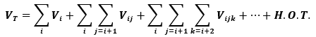
Where VT is the total variance of the model, Vi is the first order effect, or main effect, of variable i, and Vij are the second order effects due to interactions between variables i and j. The order of the effect increases with the number of the indices. The sensitivity indices are computed from these component variances by simply dividing by the total model variance.
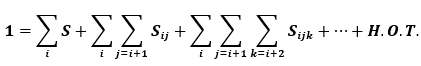
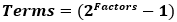
The total number of individual terms that must be computed to quantify each interaction term scales as a power law:
Due to this, it can be prohibitively computationally expensive to calculate each interaction term for even a moderate number of variables. To ease computation, generally two different indices are calculated: the first order effect index, Si, and the total effect index. The current version of the UQSA tool is set up to calculate only the first order effects of each input parameter. Future versions will implement algorithms for the computation of total effect indices. The “First Order Effect Index” is represented by the equation:
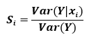
Where Var(Y│xi ) is the variance in model output varying only the parameter xi and Var(Y) is the variance in model output varying all of the parameters together. This sensitivity measure assesses the main contribution of a given parameter to the total variance of the model output and does not quantify the effects of interactions between parameters. The UQSA tool uses two methodologies to assess the first order effect index of model parameters. A Monte Carlo random sampling algorithm is employed mainly for verification of other calculation techniques in this tool but can be used for low dimensional models (less than 10 parameters) if desired. Another technique used for the computation of first order effects indices is the Fourier Amplitude Sensitivity Test (FAST) [1] which is implemented in this tool. For the FAST sensitivity analysis method, all parameter ranges are represented as cyclic functions called “search curves.” A uniform distribution search curve is used of the form [2]:

Where xmax is the maximum parameter value, xmin is the minimum parameter value, ω is the parameter frequency, and ϕ is a random phase angle from 0 to 1. When randomly sampled, this function is approximately uniformly distributed. This enables us to treat our model as a random, noisy signal. Using an N-dimensional Fourier transform, we can then filter the model output and investigate the resulting frequency spectrum.
Surrogate Modeling
For complex models that are impractical for creating an analytical model to for this tool, a Radial Basis Function Network (RBFN) surrogate model is available for approximating model performance. All inputs for the RBFN are automatically normalized to a unit hypercube; that is, within the analysis of the RBFN all parameter values have an interpreted range of 0 to 1. This normalization technique was implemented based on general practice for Gaussian Process LINK surrogate models.Example
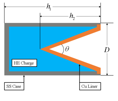
Fig 2. Simple high explosive (HE) shaped-charge with copper liner and stainless steel confinement
The following is an uncertainty quantification example using an analytical shaped-charge jet velocity problem from Meyer's textbook "Dynamic Behavior of Materials" (ISBN: 0-471-58262-X), specifically example 17.2 pg. 577. All files used are included in the UQSA download. Though effort was made to reduce the programming burden on the user, knowledge of Python programming is still required to construct model input files. Suppose you are testing a BRL 81mm shaped-charge that will produce an explosively-formed copper projectile. Using Meyer's textbook, a simple analytical model was found to be:
Where V_charge is the volume of the explosive charge, Vmetal is the volume of the copper liner, h1 is the height of the canister, h2 is the height of the copper liner cone, D is the major diameter of the canister, the ρ's are the densities of the metal and charge, M is the mass of the metal, C is the mass of the charge, V0 is the null velocity of the copper jet, GE is the Gurney Energy of the charge, β is the new angle of the liner formed by the jet, vD is the detonation velocity of the charge, v1 is the pressure stagnation point velocity, v2 is the material entrance velocity into the formed jet, α is half the included angle of the copper cone, and vjet is the velocity of the formed jet. Suppose you wanted to gauge the jet velocity as a function of the included angle of the copper liner. This would mean that height of the liner follows the equation:
The next section will show the translation of these equations into usable code for the UQSA tool.
Before running UQSA: Setting up your model file
Packaged with the tool is a folder named "model_library." This folder contains examples of code used with the UQSA tool. One such file is "simple_exponential.mdl." which we will use as a basis for building our new model. Model files (.mdl) are plain text files without special formatting. They contain Python code that is parsed to create a user model for the analysis scripts to call. The simple_exponential.mdl file contains:#PLACE USER DEFINED FUNCTIONS TO BE CALLED HERE #__startsub__ - DO NOT DELETE THIS LINE def subname(indata): ## USER MATH STUFF HERE ## outdata = indata**2.0 return outdata #__endsub__ - DO NOT DELETE THIS LINE #Write model output to main model variable for MC analysis #Only data written to 'output' will be analyzed. #__startmodel__ - DO NOT DELETE THIS LINE output = (A*exp(B*x)*x)**C
The lines starting with "#__startsub___" and "#__endsub__" are flags that tell the custom file parser where the user defined sub-functions are located. The "#__startsub__" flag must always be above the "#__endsub__" flag. The line starting with "#__startmodel__" tells the file parser where the main analysis code is located. The "#__startmodel__" flag must be below the "#__endsub__" flag. When this file is successfully read and meshed with a user parameters file, this creates operable Python model code. At the bottom of the model code section defined by "#__startmodel__" is a keyword argument "output." This is the main data storage variable that is later passed to all analysis scripts for UQSA. Only data written to "output" is analyzed. Due to program limitations, only a single scalar variable can be passed to "output." All code within the "#__startmodel__" block is automatically added to a program "for" loop to iterate over a user defined independent variable. Using this example file, the jet velocity code is constructed.
#PLACE USER DEFINED FUNCTIONS TO BE CALLED HERE
#__startsub__ - DO NOT DELETE THIS LINE
def getV0(GE,R):
	return 1000*GE*(((1.0+2.0*R)**3.0 + 1.0)/(6.0*(1.0 + R)) + R)**-0.5

def getBeta(V0,VD,alpha):
	return 2.0*np.arcsin(V0*np.cos(alpha)/(VD*2.0)) + alpha


def getV(V0,alpha,beta):
	V1 = V0*np.cos((beta-alpha)/2.0)/np.sin(beta)
	V2 = V0*(np.cos((beta-alpha)/np.tan(beta) + np.sin((beta-alpha)/2.0)))
	return V1,V2
#__endsub__ - DO NOT DELETE THIS LINE

#Write model output to main model variable for MC analysis
#Only data written to 'output' will be analyzed.
#__startmodel__ - DO NOT DELETE THIS LINE

'''
Example problem from Meyer's Dynamic Behavior of Materials
Estimation of speed for an explosively-shaped projectile
'''

# Problem geometry
alpha = theta/2.0 #rad, half included angle
h2 = D/2.0/np.tan(alpha)

# Get volumes for charge and metal
Vc = np.pi*h1*(D**2.0)/4.0 - np.pi*h2*(D**2.0)/12.0
Vm = t*(np.pi*D/2.0)*((D*D/4.0)+h2**2.0)**0.5

# Get masses for charge and metal
M = Vm*rho_m
C = Vc*rho_c
R = M/C

# Get V0
V0 = getV0(GE,R)
beta = getBeta(V0,VD,alpha)

# Get V1,V2
V1,V2 = getV(V0,alpha,beta)

# Get jet (VJ) and slug (VS) velocity
VJ = V1 + V2
VS = V1 - V2

output = VJ
The custom file parser and model wrapper routines automatically package the code so that variables do not need to be defined as arrays, so the user does not have to work with variable storage logic and reduce the amount of programming needed. For the jet velocity code, the null velocity, angle β, jet stagnation pressure point velocity (v_1), and jet material entrance velocity (v_2) were opted to be computed with sub-functions and placed in the "#__startsub__" block. Also, note that the independent variable, θ is not defined in this code. This will be supplied later within the UQSA user interface. If desired, copy and paste the above code into an empty file and name it "jet_velocity.mdl" and place it in your model library folder. Otherwise, this file is available in the UQSA download.
Before Running UQSA: Setting up your model parameter file
Copy the following into a text file and name it "simple_exponential.csv". This file is the parameter input file for "simple_exponential.mdl".#Parameter, Value, Dist Param, DISTTYPE, 0=NORMAL, 1=UNIFORM A, 1, 0.05, 0 B, 0.5, 0.005, 0 C, 2, 0.05, 0Similarly, copy the following to a text file and save it as “jet_velocity_example.csv” to create the jet velocity example problem input file.
#Parameter, Value, Dist Param, DISTTYPE, 0=NORMAL, 1=UNIFORM
GE, 2.93, 0.1465, 0
VD, 8180, 409, 0
rho_c, 1650, 0, 0
rho_m, 8900, 0, 0
D, 81, 0, 0
h1, 160, 0, 0
t, 2, 0, 0
Parameters files are comma separated values (CSV) files that contains the distribution information for each parameter of the user defined model. Now that we have a model file, the parameters file for the model can be built. Like before, we will start with one of the packaged files called "simple_exponential.csv." these files usually open by default with either Microsoft Excel on Windows or LibreOffice on Linux for easy manipulation. The file is comprised of four inputs:
- Parameter Label
- Value
- Distribution Parameter
- Distribution Type.
The UQSA GUI
Now we are ready to run the UQSA setup script. On Windows, this is generally done by double-clicking the "UQSA.py" script. For Linux systems, the script can be started by opening a terminal in the script's directory and typing the following command:python UQSA.py
From here, you should get the start-up screen. Make sure that the terminal window is visible.
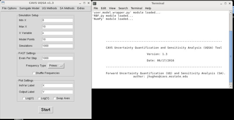
Fig 3. UQSA start screen
- File Options > Set Working Directory
- File Options > Select Model File
- File Options > Select Parameter File
- Enter simulation setup information in the "Simulation Setup", "FAST Settings," and "Plot Settings" fields
- Select Uncertainty Quantification methods using the UQ Methods drop down menu.
- Select Sensitivity Analysis methods using the SA Methods drop down menu.
Since we are working with an analytical model, the "Surrogate Model" drop down menu can be ignored.
Setting the Working Directory
Now we can begin selecting the files for our analysis. Start by clicking the drop-down menu "File Options" and then clicking "Set Working Directory." A menu will pop up asking you to select your working directory. All model analysis results will be dumped into the selected folder.Setting the Model File
Next, click "Select Model File". A file menu dialogue box will pop up. Navigate to the directory with your model file and select it. By default, the file menu dialogue looks for ".mdl" files for the UQSA script. If your file extension is different, in the "Files of Type" drop down menu select "All files."Setting the Parameter File
Now select the model parameter file by using "File Options > Select Parameter File." Navigate to the directory with your parameter file and select it. As a reminder, this file must be a comma-separated values (.csv) file in order to be properly read.Selecting Uncertainty and Sensitivity Methods
Use the respective drop-down menus for the "UQ Methods" and "SA Methods" to select methods to perform. When selected, a check mark will be displayed next to the name of the method in the drop-down menu. If you would like to test that the model and parameter files work, you can deselect all methods and have the UQSA script just run the model at the mean values supplied by the parameter file.Simulation Setup
Using the simulation setup entry fields, you can set the range of your independent variable as well as how many model steps along the curve and the number of Monte Carlo simulations. The higher the number of model steps, the longer any analysis method will take. It is good to remember that the number of model evaluations follows the formula: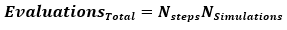
So, a model evaluated at 20 points and sampled 10,000 times will need 200,000 model evaluations. For simple models, the impact on analysis time is minimal. However, for complex models that require a high number of model points (e.g., models with numerical integration schemes), Monte Carlo analysis times could easily take hours to days depending on the power of the computer's hardware. The "Simulations" field is used by all Monte Carlo methods (Monte Carlo Uncertainty and Monte Carlo Sensitivity). The "FAST Settings" entries allow you to set the analysis parameters for the Fourier Amplitude Sensitivity Test (FAST) global sensitivity method. In general, this method is significantly faster than the Monte Carlo solution for first order sensitivity indices. "Evals per step" determines how densely the search curves for each parameter are sampled. If you do not know how many samples you want to take, set this parameter to 1. The FAST method can be thought of as a signal analysis and processing method; therefore, Nyquist's signal sampling theorem can be applied. It is implemented in the FAST algorithm as:
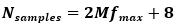
Where M is an expansion factor (set to 16 within the code) to increase the number of required samples and is the maximum parameter frequency. If your input is less than that of the Nyquist theorem, the number of samples from the Nyquist theorem is used. The "Frequency Type" drop down menu can be used to select a frequency generator. The "Primes" setting generally produces better results over "Platonians." The "Shuffle Frequencies" check box can be used to force the frequencies generated to be randomly shuffled before being assigned to a parameter. This can be used to ensure that each subsequent run of the FAST method produces comparable results, regardless of the assigned parameter frequencies. These inputs are only necessary when the FAST sensitivity method is selected to run. Lasty, the "Plot Settings" entries can be used to set the independent variable and output variable axis labels. Since the plotting method calls the matplotlib module, these fields accept LaTeX format text if desired. To enable LaTeX formatting, use the dollar symbol ($) around the text to format. For example:
IndVar Label: Included Angle, $\theta \left( rad \right)$
Output Label: Jet Velocity, $V_{j} \left( \frac{m}{s} \right)$
This will display on the plot as “Included Angle,θ(rad)” and “Jet Velocity,Vj (m/s)”. By default, the independent variable is plotted along the x-axis and the output variable along the y-axis. If you would like to flip the axes, select "Swap X/Y". If either axis needs to be log formatted select "Log(X)" and/or "Log(Y)." Below are the UQSA settings which will be used to run this example problem.
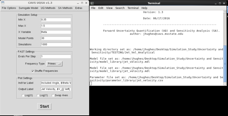
Fig 4. UQSA settings for jet velocity example problem
Results
For the sake of the example, ensure that the "Monte Carlo Analysis" uncertainty method and the "FAST First Order Effects Indices" sensitivity method are active. Once the UQSA settings are to your liking, just hit the "Start" button to start the analysis. The terminal window will update as each new analysis method is run. The terminal window will also display any errors that may result from a bad user model file. Typically, errors are trivial programming mistakes when writing the model code or an undefined variable. In the latter case, this is generally if the user used the wrong variable name for the parameter file.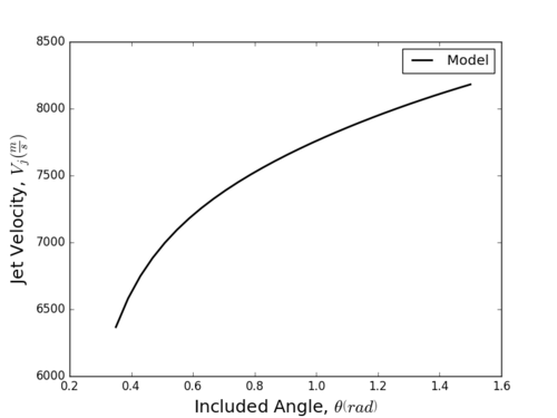
Fig 5. Results From Included Parameter Sets Without Uncertainty and Sensitivity Options Selected
Any errors with running the model will be output to the terminal window. Address any errors that arise and try again. Unfortunately, since Python stores functions in memory in case they are needed again, if you need to make changes to your model file you must restart the tool for these changes to take effect.
Forward Uncertainty Propagation: Monte Carlo Simple Random Sampling
A Monte Carlo (MC) Simple Random Sampling method was used for forward propagation of uncertainty through our model.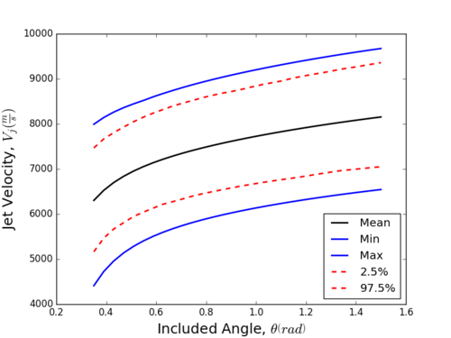
Fig 6. Uncertainty Results from the Monte Carlo Analysis
From can be seen from the uncertainty bands (the 2.5% and 97.5% lines), it looks like our data is approximately normally distributed since the mean is approximately centered between our uncertainty bands. This can be confirmed by analyzing the histogram results for each step in the "Monte Carlo" output folder in your working directory (and for a more robust determination, an Anderson-Darling hypothesis test). This representation of our data can give us an idea as to how precise our model is with respect to the uncertainty going in; however, it cannot tell us which parameters controlled the uncertainty. Next, we will look at the FAST method's computed sensitivity values to determine the most influential parameters.
Global Sensitivity Analysis: Fourier Amplitude Sensitivity Test (FAST)
As previously stated, the FAST method allows us to turn our sensitivity analysis problem into a random, noisy signal Fourier filtering problem. By analyzing the coefficients of a discrete Fourier transform, we can determine which frequency (and in turn, parameter) accounts for the most variation in model output. Below is a graph of the computed sensitivity measures for each parameter as a function of the included angle.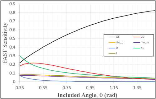
Fig 7. FAST Sensitivity of Input Parameters
From this graph, it can be seen that the GE term (the high explosive's Gurney Energy) controls the uncertainty for the majority of the predicted jet velocity, followed by the high explosive's detonation velocity (VD), and lastly the overall length of the charge (h1). Using this information, we can target which parameters we need to more precisely control or measure in experiments.