LAMMPS Stacking | Code Repository | ICME

Abstract

his example shows how to run an atomistic simulation to generate the generalized stacking fault (GSF) energy curve for FCC metals. This example uses a parallel molecular dynamics code, LAMMPS^[1]. Excel is used to plot the energy-displacement and Ovito is used to visualize the simulation.

Author(s): Phillip M. Spear*

Advisor(s): Firas Akasheh*, Mark A. Tschopp

(*) Mechanical Engineering Department, Tuskegee University, Tuskegee, AL 36088

Corresponding Author: Mark A. Tschopp

Input

Description of Simulation

The generalized stacking fault energy curve is obtained by rigidly displacing two halves of a crystal on a (111) plane along a <112> direction in that plane. As the displacement proceeds, the energy of the crystal changes as the atoms slip by each other. The potential used here is the Mishin et al. (1999) aluninum potential.^[2] This molecular dynamics simulation first generates a simulation cell with fcc atoms of orient [112] in the x, [-110] in the y, and [-1-11] in the z direction and a total of 6,995 atoms are created. The cell size will be 10 lattice units in the x and y directions and 40 lattice units in the z direction. Note that the units in the x and y direction are modified to reflect the different periodicit boundaries of the structure in the corresponding.The top half of the crystal is shifted in the xy plane along the x direction. With this scheme, the boundary conditions used are periodic, periodic and free surface in the x, y, and z directions, respectively. After the displacement in the x direction is made, the crystal is allowed to relax in the z direction and the energy is calculated and then dumped into the dump.comp.* file.

LAMMPS input script for FCC

This input script was run using the December 21 2011 version of LAMMPS. Changes in some commands in more recent versions may require revision of the input script. To run this script, store it in "in.stack_fault.txt" and then use the "lmp_win_no-mpi.exe < in.stack_fault.txt" in a Windows environment where "lmp_win_no-mpi.exe" refers to the LAMMPS executable.

# Input file for Stack Fault Energy surface of Aluminum
# Phillip Spear, 2012

# ------------------------ INITIALIZATION ----------------------
units metal
dimension 3
boundary p p s
atom_style atomic
variable latparam1 equal 4.05

variable xdim equal ${latparam1}*sqrt(6)/2*10
variable ydim equal ${latparam1}*sqrt(2)/2*10

# ----------------------- ATOM DEFINITION ----------------------
lattice fcc ${latparam1}
region 1 block 0 ${xdim} 0 ${ydim} 0 20 
region 2 block 0 ${xdim} 0 ${ydim} 20 40
region whole block 0 ${xdim} 0 ${ydim} 0 200 units box
create_box 1 whole
lattice fcc ${latparam1} orient x 1 1 2 orient y -1 1 0 orient z -1 -1 1
create_atoms 1 region 1
lattice fcc ${latparam1} orient x 1 1 2 orient y -1 1 0 orient z -1 -1 1
create_atoms 1 region 2

# ----------------------- FORCE FIELDS -----------------------
pair_style eam/alloy
pair_coeff * * Al99.eam.alloy Al

# ------------------------- SETTINGS --------------------------
group top region 1
group bot region 2

# ------------------------- Displacement -----------------------
displace_atoms bot move -1.0 0.0 0.0 units box
compute peratom all pe/atom
compute eatoms all reduce sum c_peratom

# Dump to comp  for Ovito post processing 
dump 1 all custom 1 dump.comp.* id type xs ys zs c_peratom fx fy fz

thermo 1
thermo_style custom step pe c_eatoms

fix 1 all setforce 0 0 NULL

min_style cg
minimize 1e-10 1e-10 1 1

# SIMULATION DONE
#print ${x}
print "All done"

Output

LAMMPS logfile

The log.lammps file should look like this below

LAMMPS (21 Dec 2011)
# Input file for Stack Fault Energy surface of Aluminum
# Phillip Spear, 2012

# ------------------------ INITIALIZATION ---------------------
units 		metal
dimension	3
boundary	p	p	s
atom_style	atomic
variable latparam1 equal 4.05
#variable xlattice equal ${latparam1}*sqrt(6)/2
#variable ylattice equal ${latparam1}*sqrt(2)/2

variable xdim equal ${latparam1}*sqrt(6)/2*10
variable xdim equal 4.05*sqrt(6)/2*10
variable ydim equal ${latparam1}*sqrt(2)/2*10
variable ydim equal 4.05*sqrt(2)/2*10

# ----------------------- ATOM DEFINITION ---------------------
lattice		fcc ${latparam1}
lattice		fcc 4.05
Lattice spacing in x,y,z = 4.05 4.05 4.05
region		1 block 0 ${xdim} 0 ${ydim} 0 20
region		1 block 0 49.60216729 0 ${ydim} 0 20
region		1 block 0 49.60216729 0 28.63782464 0 20
region		2 block 0 ${xdim} 0 ${ydim} 20 40
region		2 block 0 49.60216729 0 ${ydim} 20 40
region		2 block 0 49.60216729 0 28.63782464 20 40
region		whole block 0 ${xdim} 0 ${ydim} 0 162 units box
region		whole block 0 49.60216729 0 ${ydim} 0 162 units box
region		whole block 0 49.60216729 0 28.63782464 0 162 units box
create_box	1 whole
Created orthogonal box = (0 0 0) to (49.6022 28.6378 162)
  1 by 1 by 1 MPI processor grid
lattice	fcc ${latparam1} orient x 1 1 2 orient y -1 1 0 orient z -1 -1 1
lattice	fcc 4.05 orient x 1 1 2 orient y -1 1 0 orient z -1 -1 1
Lattice spacing in x,y,z = 6.61362 5.72756 7.01481
create_atoms	1 region 1
Created 6959 atoms
lattice	fcc ${latparam1} orient x 1 1 2 orient y -1 1 0 orient z -1 -1 1
lattice	fcc 4.05 orient x 1 1 2 orient y -1 1 0 orient z -1 -1 1
Lattice spacing in x,y,z = 6.61362 5.72756 7.01481
create_atoms	1 region 2
Created 6995 atoms


# ----------------------- FORCE FIELDS ------------------------
pair_style	eam/alloy
pair_coeff	* * Al99.eam.alloy Al

# ------------------------- SETTINGS --------------------------
group top region 1
6959 atoms in group top
group bot region 2
6995 atoms in group bot



displace_atoms bot move -1.0 0.0 5.0 units box
compute peratom all pe/atom
compute eatoms all reduce sum c_peratom

# Dump to comp  for Ovito post processing 
dump 1 all custom 1 dump.comp.* id type xs ys zs c_peratom fx fy fz

thermo 1
thermo_style custom step pe c_eatoms

fix 1 all setforce 0 0 NULL

min_style cg
minimize 1e-10 1e-10 1 1
WARNING: Resetting reneighboring criteria during minimization (min.cpp:167)
Memory usage per processor = 11.5713 Mbytes
Step PotEng eatoms 
       0   -46556.082   -46556.082 
       1   -46556.501   -46556.501 
Loop time of 1.44408 on 1 procs for 1 steps with 13954 atoms

Minimization stats:
  Stopping criterion = max force evaluations
  Energy initial, next-to-last, final = 
        -46556.0821773     -46556.0821773     -46556.5012397
  Force two-norm initial, final = 2.1518 1.04566
  Force max component initial, final = 0.375727 0.189924
  Final line search alpha, max atom move = 0.133075 0.0252742
  Iterations, force evaluations = 1 2

Pair  time (%) = 0.322017 (22.2991)
Neigh time (%) = 0 (0)
Comm  time (%) = 0.00200115 (0.138576)
Outpt time (%) = 0 (0)
Other time (%) = 1.12006 (77.5624)

Nlocal:    13954 ave 13954 max 13954 min
Histogram: 1 0 0 0 0 0 0 0 0 0
Nghost:    15056 ave 15056 max 15056 min
Histogram: 1 0 0 0 0 0 0 0 0 0
Neighs:    941163 ave 941163 max 941163 min
Histogram: 1 0 0 0 0 0 0 0 0 0

Total # of neighbors = 941163
Ave neighs/atom = 67.4475
Neighbor list builds = 0
Dangerous builds = 0


######################################
# SIMULATION DONE
#print ${x}
print "All done"All done

LAMMPS dumpfile

The following is an example of one of the dumpfiles poduced by the simulation

ITEM: TIMESTEP
0
ITEM: NUMBER OF ATOMS
16526
ITEM: BOX BOUNDS pp pp ss
0 40.5
0 40.5
-0.0001 161.341
ITEM: ATOMS id type xs ys zs c_peratom fx fy fz 
1 1 0 0.0707107 6.19806e-007 -3.02107 -0.507551 -0.161139 0.211959 
2 1 0.0204124 0.0353553 0.0144934 -3.40036 -0.509427 -0.0618367 0.382914 
3 1 0.0204124 0.106066 0.0144934 -3.18184 -0.521879 -0.043691 0.320027 
4 1 0 0 6.19806e-007 20.2456 43.1252 69.3146 0.284397 
5 1 0.0612372 0.0353553 6.19806e-007 -3.07992 0.0151763 -0.155602 -0.0718626 
10 1 0.0612372 0.106066 6.19806e-007 -2.75558 0.221845 0.129318 0.0760658 
50 1 0.0816497 0.0707107 0.0144934 -3.28357 0.186384 0.113913 -0.0219166 
53 1 0.0816497 0 0.0144934 10.5204 0.295648 60.6059 -0.180713 
54 1 0.122474 0 6.19806e-007 -2.7993 0.189235 -0.175251 0.186386 
55 1 0.142887 0.0353553 0.0144934 -3.3544 0.00659385 -0.118225 0.110351 
68 1 0.142887 0.106066 0.0144934 -3.29271 -0.0153932 -0.00281737 -0.0885542 
70 1 0.122474 0.0707107 6.19806e-007 -2.88973 0.0471537 0.184517 0.0487032 
71 1 0.183712 0.0353553 6.19806e-007 -3.04259 -0.0275901 -0.157453 0.0477017 
72 1 0.183712 0.106066 6.19806e-007 -2.89648 -0.132644 -0.0136961 0.0622947 
194 1 0.204124 0 0.0144934 10.529 0.0494405 60.6236 0.101715 
219 1 0.204124 0.0707107 0.0144934 -3.37019 0.0688223 0.105116 0.0661885 
220 1 0.244949 0.0707107 6.19806e-007 -3.07376 -0.0116489 -0.00299865 -0.0328375 
221 1 0.265361 0.0353553 0.0144934 -3.41371 0.021542 -0.103852 0.108885 
222 1 0.265361 0.106066 0.0144934 -3.32621 -0.000735514 -0.140739 0.0401943 
....

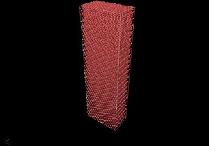
This is a perspective view of the simulation cell with atoms.

Post-Processing

Visualization

The simulation can be visualized using Ovito^[3] To do so, open the Ovito program and select the import data tab. Now go to the directory in which you ran the simulation. Locate the first dumpfile, which would be dump.comp.0 in this case, that results from the simulation. Select open and on the next page choose the option to use the wild card name, dump.comp*, to load all the dump files. Then choose auto-assign columns and select OK. Use the play, forward and backward skip button located at the bottom of the program to view the different snapshots.

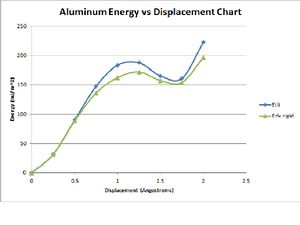
This is a chart of Evergy at each given displacement.

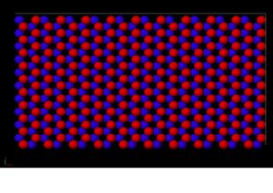
Figure 1. This is a snapshot of the plane before displacement. The red atoms are on top while the blue atoms are on bottom.

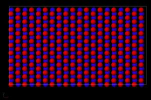
Figure 2. This is a snapshot of the plane that is displaced at 1.

Acknowledgements

The author and first advisor would like to acknowledge the support to this work by the National Science Foundation, HBCUUP-RIA program, Program Manager Dr. Claudia Rankins, Award No. HRD-1137587. Additionally, the technical and logistical support of CAVS and HPC2 of Mississippi State University is acknowledged. The corresponding author author would like to acknowledge funding for the overarching EVOWiki project through the Department of Energy.

References

↑ S. Plimpton, "Fast Parallel Algorithms for Short-Range Molecular Dynamics," J. Comp. Phys., 117, 1-19 (1995). (http://www.sciencedirect.com/science/article/pii/S002199918571039X)
↑ Y. Mishin, D. Farkas, M.J. Mehl, and D.A. Papaconstantopoulos, "Interatomic potentials for monoatomic metals from experimental data and ab initio calculations," Phys. Rev. B 59, 3393 (1999).
↑ A.Stukowski, "Visualization and analysis of atomistic simulation data with OVITO - the Open Visualization Tool," Modelling Simul. Mater. Sci. Eng. 18 (2010), 015012.(http://ovito.org/)

Integrated Computational Materials Engineering (ICME)

LAMMPS Stacking Fault Energy