
Integrated Computational Materials Engineering (ICME)
LAMMPS Polymer
Abstract
In this tutorial Molecular dynamics simulation in LAMMPS is used to show what happens to a polymer chain at a certain temperature after some time. Chain's movement is caused by a molecular forces between atoms in the chain and by temperature of the chain. This factors are modeled in LAMMPS in order to show the behavior of this polymer chain. The chain was previously prepared in MATLAB. It contains 100 atoms with bound between neighbor atoms. During the simulation, firstly, the chain was left for do deform freely under the molecular forces and a random atomic fluctuation due to the temperature. After that the chain was minimized to find it's minimal energy condition. The tutorial explains basic LAMMPS commands and shows how to make a movie using AtomEye and ImageJ.
Author(s): Dmitry I. Zhuk, Mark A. Tschopp
Corresponding Author: Mark Tschopp
Input File
The polymer chain of 100 atoms was specially prepared in MATLAB. The atom's Z coordinate does not varies much, all of them are within 2 Å. The distance between atoms is about 1.5 Å. Basically, the chain goes from left upper to right lower corner of the box. At the right you can see the picture of the initial condition of the chain.
The data file is shown below and available for download here: PE_cl100.txt
# Model for PE

     100     atoms
      99     bonds
      98     angles
      97     dihedrals

         1     atom types
         1     bond types
         1     angle types
         1     dihedral types

    0.0000   158.5000 xlo xhi
    0.0000   158.5000 ylo yhi
    0.0000   100.0000 zlo zhi

Masses

         1          14.02

Atoms

         1         1         1    5.6240    5.3279   51.6059
         2         1         1    7.4995    7.4810   50.2541
         3         1         1    8.2322    8.0236   51.2149
         4         1         1    9.6108    9.9075   51.7682
         5         1         1   11.5481   11.3690   50.4167
         6         1         1   12.9409   13.4562   50.2481
         7         1         1   14.4708   14.8569   50.0868
         8         1         1   16.1916   16.4790   50.5665
         9         1         1   17.1338   17.6853   51.8189
        10         1         1   19.1109   19.4000   50.3869

...

Bonds

         1         1         1         2
         2         1         2         3
         3         1         3         4
         4         1         4         5
         5         1         5         6
         6         1         6         7
         7         1         7         8
         8         1         8         9
         9         1         9        10
        10         1        10        11

...

Angles

         1         1         1         2         3
         2         1         2         3         4
         3         1         3         4         5
         4         1         4         5         6
         5         1         5         6         7
         6         1         6         7         8
         7         1         7         8         9
         8         1         8         9        10

...

Dihedrals

         1         1         1         2         3         4
         2         1         2         3         4         5
         3         1         3         4         5         6
         4         1         4         5         6         7
         5         1         5         6         7         8
         6         1         6         7         8         9
         7         1         7         8         9        10
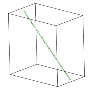
Figure 1. Not-deformed polymer chain.
Here, the first section defines the numbers of atoms, bonds, angles and dihedrals. Lower you can see the types and the box sizes. Below that are the simulation box sizes.
Then comes the Atoms section. The first column is the atom number, then comes the atom type and some other information not used in this tutorial. Last three columns is the atom's x, y and z coordinates correspondingly.
In the Angle section listed the angles between atoms. First column is the angle number, second - angle ID, then comes the atom's number between which the angle is defined. Example of the distribution of the atoms can be seen on Figure 2. Dihedrals are a little bit more complicated. To define a diherdal four atoms are needed. Syntax are pretty much similar to the angles section. The only difference is that one more atom is needed to define a dihedral. Basically, the dihedral angle is the angle between the planes formed by 2 groups of 3 neighbor atoms. You see the example on Figure 3.
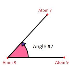
Figure 2. Angles between atoms defined in LAMMPS.
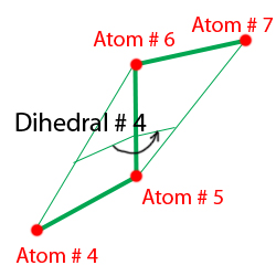
Figure 3. Angles between atoms defined in LAMMPS.
LAMMPS Script
Below is the script used for the actual simulation. This input script was run using the Aug 2015 version of LAMMPS. Changes in some commands in more recent versions may require revision of the input script. This script runs the simulation with the previously discussed data file.
#####################################################
#                                                   #
#                                                   #
# Filename: in.deform.polychain.txt                 #
# Author: Mark Tschopp, 2010                        #
#                                                   #
# The methodology outlined here follows that from   #
# Hossain, Tschopp, et al. 2010, Polymer.  Please   #
# cite accordingly. The following script requires   #
# a LAMMPS data file containing the coordinates and #
# appropriate bond/angle/dihedral lists for each    #
# united atom.                                      #
#                                                   #
# Execute the script through:                       #
# lmp_exe < in.deform.polychain.txt                 #
#                                                   #
#####################################################

# VARIABLES
variable fname index PE_cl100.txt
variable simname index PE_cl100

# Initialization
units		real
boundary	f f f
atom_style	molecular
log 		log.${simname}.txt
read_data	${fname}

# Dreiding potential information
neighbor	0.4 bin
neigh_modify	every 10 one 10000
bond_style      harmonic
bond_coeff	1 350 1.53
angle_style     harmonic
angle_coeff	1 60 109.5
dihedral_style	multi/harmonic
dihedral_coeff	1 1.73 -4.49 0.776 6.99 0.0
pair_style	lj/cut 10.5
pair_coeff	1 1 0.112 4.01 10.5

compute csym all centro/atom fcc
compute peratom all pe/atom


#####################################################
# Equilibration (Langevin dynamics at 5000 K)

velocity 	all create 5000.0 1231
fix		1 all nve/limit 0.05
fix		2 all langevin 5000.0 5000.0 10.0 904297
thermo_style	custom step temp
thermo          10000
timestep	1
run		1000000
unfix 1
unfix 2
write_restart 	restart.${simname}.dreiding1


#####################################################
# Define Settings
compute eng all pe/atom
compute eatoms all reduce sum c_eng

#####################################################
# Minimization

dump 		1 all cfg 6 dump.comp_*.cfg mass type xs ys zs c_csym c_peratom fx fy fz

reset_timestep 0
fix 1 all nvt temp 500.0 500.0 100.0
thermo 20
thermo_style custom step pe lx ly lz press pxx pyy pzz c_eatoms
min_style cg
minimize 1e-25 1e-25 500000 1000000


print "All done"
In general, this script does equilibration and minimization to the polymer chain. Polymer chain data file named 'PE_cl100.txt' should be the same directory. Line "dump 1 all cfg 6 dum..." used to output information during simulation can be moved before the equilibration part of the script to output the process of equilibration. Please note that you need to change a time step for a dump command otherwise it will give too many or very few dump files. It may be reasonable to choose a timestep of 10,000 for equilibration and 6 for minimization. That will give about 100 files for each step.
# VARIABLES
variable fname index PE_cl100.txt
variable simname index PE_cl100

# Initialization
units		real
boundary	f f f
atom_style	molecular
log 		log.${simname}.txt
read_data	${fname}
This part is just opens the data file, defines the boundary conditions, units, logfile's name, etc.
# Dreiding potential information
neighbor	0.4 bin
neigh_modify	every 10 one 10000
bond_style      harmonic
bond_coeff	1 350 1.53
angle_style     harmonic
angle_coeff	1 60 109.5
dihedral_style	multi/harmonic
dihedral_coeff	1 1.73 -4.49 0.776 6.99 0.0
pair_style	lj/cut 10.5
pair_coeff	1 1 0.112 4.01 10.5
In this section goes the information about the bonds, angles, dihedrals in a chain. Bond_style and bond_coeff defines the type on the force field between atoms and a magnitude of this fields. "1" here corresponds to the second column of the "Bonds" section of the data file. Thus, every atom pair with "1" in the second column will be having such properties during the simulation. Similar goes to the angles and dihedrals. Angle_* and dihedral_* lines defines the angles and dihedral angles between atoms in the polymer chain. Pair_* commands used to define pair potentials between atoms that are within a cutoff distance. More about this commands and a parameters can be found at SANDIA website: https://lammps.sandia.gov/doc/Section_commands.html#cmd_5
compute csym all centro/atom fcc
compute peratom all pe/atom
his commands are used to define which properties are to be calculated during the simulation. For example, "pe/atom" simply means to calculate the potential energy for each atom. Information about other possible properties to calculate can be found here.
# Equilibration (Langevin dynamics at 5000 K)

velocity 	all create 5000.0 1231
fix		1 all nve/limit 0.05
fix		2 all langevin 5000.0 5000.0 10.0 904297
thermo_style	custom step temp
thermo          10000
timestep	1
run		1000000
unfix 1
unfix 2
write_restart 	restart.${simname}.dreiding1
The equilibration step allows the chain to deform freely under the temperature driven movements of the atoms. Velocity command add the temperature to the chain. Fix command performs the check of the system every time step and updates the velocity and positions of the atoms. Thermo commands defines thermo output during the simulation. Run command stars the dynamic transformation.
#####################################################
# Minimization

dump 		1 all cfg 6 dump.comp_*.cfg id type xs ys zs c_csym c_peratom fx fy fz

reset_timestep 0
fix 1 all nvt temp 500.0 500.0 100.0
thermo 20
thermo_style custom step pe lx ly lz press pxx pyy pzz c_eatoms
min_style cg
minimize 1e-25 1e-25 500000 1000000
The other step in the program is the minimization. It finds the minimum energy condition for such configuration. The parameters for minimize command includes: stopping tolerance for energy, stopping tolerance for force, max iterations of minimizer and max number of force/energy evaluations. Where stopping tolerance for energy being the first parameter and the max number of force/energy evaluations the last one.
LAMMPS Logfile
Here is the logfile produced by LAMMPS during the simulation. Note that the temperature during the equilibration does not concave and just randomly changes over time. On the other hand, the potential energy during the minimization lowers over time until it reaches the minimum for this configuration within a tolerance.
read_data	${fname}
read_data	PE_cl100.txt
  1 = max bonds/atom
  1 = max angles/atom
  1 = max dihedrals/atom
  orthogonal box = (0 0 0) to (158.5 158.5 100)
  2 by 2 by 1 processor grid
  100 atoms
  99 bonds
  98 angles
  97 dihedrals
  2 = max # of 1-2 neighbors
  2 = max # of 1-3 neighbors
  4 = max # of 1-4 neighbors
  6 = max # of special neighbors

# Dreiding potential information
neighbor	0.4 bin
neigh_modify	every 10 one 10000
bond_style      harmonic
bond_coeff	1 350 1.53
angle_style     harmonic
angle_coeff	1 60 109.5
dihedral_style	multi/harmonic
dihedral_coeff	1 1.73 -4.49 0.776 6.99 0.0
pair_style	lj/cut 10.5
pair_coeff	1 1 0.112 4.01 10.5

compute csym all centro/atom fcc
compute peratom all pe/atom


#####################################################
# Equilibration (Langevin dynamics at 5000 K)

velocity 	all create 5000.0 1231
fix		1 all nve/limit 0.05
fix		2 all langevin 5000.0 5000.0 10.0 904297
thermo_style	custom step temp
thermo          10000
timestep	1
run		1000000
Memory usage per processor = 5.96847 Mbytes
Step Temp
       0         5000
   10000    4503.8382
   20000    4389.5108
   30000    4137.4417
   40000    5341.7194
   50000    4458.9062
   60000    5377.3337
   70000    5004.3444
   80000    4338.4843
   90000    4691.7776
  100000    4733.5682
  110000    4701.5107
  120000    4855.5683
  130000    4477.8402
  140000    4538.7404
  150000    4588.4541
  160000    4862.2936
  170000    4684.8557
  180000    4485.3563
  190000    4759.6888
  200000     5381.965
  210000    5137.9384
  220000    4812.9015
  230000    4628.1747
  240000    4645.6596
  250000    4913.3042
  260000    5404.8637
  270000    4420.5497
  280000     5357.551
  290000    5009.1386
  300000    4610.7359
  310000    4752.3123
  320000    4358.3474
  330000    4961.3549
  340000    4317.1413
  350000    4154.0022
  360000    5339.4602
  370000     4460.511
  380000    4997.8213
  390000    4354.7411
  400000    4797.0648
  410000     4830.892
  420000    5087.6876
  430000    4723.8778
  440000    4629.8021
  450000    4976.1032
  460000    4609.4548
  470000    5019.8023
  480000    4446.1004
  490000    4862.2646
  500000     5026.155
  510000     4431.281
  520000    4391.5373
  530000    4214.6362
  540000    4846.1485
  550000    4807.4181
  560000    4488.3661
  570000    5360.1736
  580000    5071.4535
  590000     4463.498
  600000    4555.1718
  610000    5114.4069
  620000    4699.2292
  630000    5142.6987
  640000    4479.5147
  650000    4671.0304
  660000    4564.5161
  670000    4265.3884
  680000    4814.3015
  690000    4964.3923
  700000    5121.2814
  710000    5230.1069
  720000    4297.1403
  730000    4433.7983
  740000    5176.7691
  750000    4783.2431
  760000    4792.0254
  770000    4318.1008
  780000    5279.5916
  790000    4970.3985
  800000    4163.3936
  810000    5014.5128
  820000    4423.9304
  830000    4860.6778
  840000    4502.2809
  850000    4738.7186
  860000    4585.4628
  870000    4851.0205
  880000    4747.5203
  890000    4511.0158
  900000    4841.8463
  910000    5075.7912
  920000    5070.3709
  930000    4343.2652
  940000    4743.7859
  950000    4020.8883
  960000    4671.5891
  970000    4446.4685
  980000     4448.264
  990000    4507.5559
 1000000    4873.6706
Loop time of 36.1922 on 4 procs for 1000000 steps with 100 atoms

Pair  time (%) = 4.03491 (11.1486)
Bond  time (%) = 8.30473 (22.9462)
Neigh time (%) = 1.95553 (5.40319)
Comm  time (%) = 19.297 (53.3182)
Outpt time (%) = 0.00102639 (0.00283595)
Other time (%) = 2.59897 (7.18103)

Nlocal:    25 ave 39 max 5 min
Histogram: 1 0 0 0 0 1 0 0 1 1
Nghost:    45.75 ave 62 max 25 min
Histogram: 1 0 0 0 0 1 0 1 0 1
Neighs:    267.75 ave 425 max 44 min
Histogram: 1 0 0 0 1 0 0 0 1 1
FullNghs: 0 ave 0 max 0 min
Histogram: 4 0 0 0 0 0 0 0 0 0

Total # of neighbors = 1071
Ave neighs/atom = 10.71
Ave special neighs/atom = 5.88
Neighbor list builds = 100000
Dangerous builds = 100000
unfix 1
unfix 2
write_restart 	restart.${simname}.dreiding1
write_restart 	restart.PE_cl100.dreiding1


#####################################################
# Define Settings
compute eng all pe/atom
compute eatoms all reduce sum c_eng

#####################################################
# Minimization

dump 		1 all cfg 6 dump.comp_*.cfg id type xs ys zs c_csym c_peratom fx fy fz

reset_timestep 0
fix 1 all nvt temp 500.0 500.0 100.0
thermo 20
thermo_style custom step pe lx ly lz press pxx pyy pzz c_eatoms
min_style cg
minimize 1e-25 1e-25 500000 1000000
WARNING: Resetting reneighboring criteria during minimization
Memory usage per processor = 6.81045 Mbytes
Step PotEng Lx Ly Lz Press Pxx Pyy Pzz eatoms
       0    1237.2398        158.5        158.5          100    16.181003    10.716166    11.032966    26.793875    1237.2398
      20    93.175603        158.5        158.5          100    23.387346    19.859621     23.64755    26.654868    93.175603
      40    63.587362        158.5        158.5          100    25.830375    21.672133    27.047328    28.771665    63.587362
      60    54.741088        158.5        158.5          100    26.066912    21.364531      27.7035    29.132705    54.741088
      80    48.917554        158.5        158.5          100     25.87727    20.908929    27.620402    29.102479    48.917554
     100    45.293817        158.5        158.5          100    26.386696    21.757562    27.905252    29.497275    45.293817
     120    41.459225        158.5        158.5          100    25.974718    20.775913    27.911315    29.236928    41.459225
     140    37.876111        158.5        158.5          100    25.799883    20.794051    27.553625    29.051972    37.876111
     160    36.701952        158.5        158.5          100    25.852641    20.951326    27.544375    29.062221    36.701952
     180     35.07739        158.5        158.5          100    26.004914    21.057098    27.774282    29.183362     35.07739
     200    33.877666        158.5        158.5          100    25.961315     21.11421    27.590146     29.17959    33.877666
     220     31.12208        158.5        158.5          100    23.995326    19.308908     24.96515    27.711921     31.12208
     240    28.809216        158.5        158.5          100    25.831303    21.277521    27.270668    28.945719    28.809216
     260     26.02543        158.5        158.5          100    25.951859     21.58113    27.157947    29.116498     26.02543
     280    23.070199        158.5        158.5          100    26.005868    21.781819    27.222861    29.012922    23.070199
     300    20.013665        158.5        158.5          100    25.453848    20.749404    26.676606    28.935533    20.013665
     320    18.738385        158.5        158.5          100    25.954677    21.603359    27.136183    29.124488    18.738385
     340    16.749844        158.5        158.5          100    25.789221    21.322696     27.03715    29.007817    16.749844
     360      15.8834        158.5        158.5          100    25.985101    21.659604    27.170167    29.125532      15.8834
     380    14.987185        158.5        158.5          100    25.977784    21.397522    27.357437    29.178393    14.987185
     400    14.517165        158.5        158.5          100     25.95897     21.55348    27.296561    29.026868    14.517165
     420      13.7945        158.5        158.5          100    26.006995    21.535186    27.281645    29.204153      13.7945
     440    12.512098        158.5        158.5          100    25.840513     21.28497    27.217437    29.019132    12.512098
     460    12.290892        158.5        158.5          100    25.924928    21.357401    27.298119    29.119263    12.290892
     480    10.775174        158.5        158.5          100    25.830121    21.201044    27.158886    29.130434    10.775174
     500    10.218356        158.5        158.5          100    25.614842      21.0218    26.893606     28.92912    10.218356
     520    9.8614258        158.5        158.5          100     25.93082    21.345743    27.320707    29.126011    9.8614258
     540    9.1390877        158.5        158.5          100    25.893538     21.32844    27.283388    29.068787    9.1390877
     560    8.5527184        158.5        158.5          100    25.954932    21.387239    27.355923    29.121632    8.5527184
     580    8.1607915        158.5        158.5          100    25.865475     21.24017    27.270322    29.085934    8.1607915
     600    7.8012324        158.5        158.5          100    25.950545    21.404499    27.375776    29.071362    7.8012324
     620    7.6152706        158.5        158.5          100    25.937275    21.370367    27.342438    29.099019    7.6152706
     640    7.3593621        158.5        158.5          100    25.940706    21.344493    27.415647    29.061979    7.3593621
     656    7.2144567        158.5        158.5          100    25.915345    21.326291    27.308608    29.111136    7.2144567
Loop time of 0.712466 on 4 procs for 656 steps with 100 atoms

Minimization stats:
  Stopping criterion = linesearch alpha is zero
  Energy initial, next-to-last, final =
         1237.23980569      7.21445672663      7.21445672663
  Force two-norm initial, final = 1373.33 1.10527
  Force max component initial, final = 285.91 0.235955
  Final line search alpha, max atom move = 6.31527e-09 1.49012e-09
  Iterations, force evaluations = 656 3308

Pair  time (%) = 0.0280486 (3.93683)
Bond  time (%) = 0.0298776 (4.19355)
Neigh time (%) = 0.00120121 (0.168599)
Comm  time (%) = 0.05711 (8.01581)
Outpt time (%) = 0.359286 (50.4284)
Other time (%) = 0.236944 (33.2568)

Nlocal:    25 ave 41 max 4 min
Histogram: 1 0 0 0 1 0 0 0 1 1
Nghost:    47.25 ave 65 max 26 min
Histogram: 1 0 0 0 0 1 1 0 0 1
Neighs:    287.25 ave 507 max 30 min
Histogram: 1 0 0 1 0 0 0 1 0 1
FullNghs: 573 ave 992 max 47 min
Histogram: 1 0 0 0 1 0 0 1 0 1

Total # of neighbors = 2292
Ave neighs/atom = 22.92
Ave special neighs/atom = 5.88
Neighbor list builds = 51
Dangerous builds = 0


print "All done"
All done
LAMMPS dump files
Also, the dump files have been produced during the simulation. The can be used to produce a movie.
Movie
- Go to AtomEye website.
- Click on Download, this will take you to the raw binary files.
- Download the A.i686 version by right-clicking on the link and "Save Target As..." to one of your directories.
- Rename the downloaded file as A by typing "cp A.i686 A". A will be the executable.
- Using UNIX, run "chmod A 755" on the file to change this to an executable.
- To test, you need to save a CFG file as well, such as cnt8x3.cfg. Try running using "./A cnt8x3.cfg".
- Go to ImageJ website.
- Download the appropriate version for Windows, LINUX, or MAC
- Visualize the dumpfile in AtomEye by typing the following command, "/A dump.tensile_0.cfg" (UNIX).
- Visualize the dumpfile in AtomEye by typing the following command, "/A dump.tensile_0.cfg" (UNIX).
- Use Alt+0 to activate centrosymmetric (csym) view.
- Adjust threshold, or set of atoms to view, by using Shift+T. This will allow creation of a set for the current parameter (in this case, csym). Please note that you need to adjust both lower and higher thresholds unless the atoms from following images that exceeds maximum value for the first one will be not shown. You can make it 5 or 10.
- Make atoms with values outside of the threshold invisible by using Ctrl+A.
- Press 'y' within AtomEye to produce an animation script.
- The folder "Jpg" now contains snapshots of all dumpfiles.
- Open ImageJ
- Drag the folder Jpg into ImageJ
- Select "Convert to RGB" to keep the color from the AtomEye images.
- Choose "yes" to load a stack.
- Adjust the size as needed (Image/Adjust/Size)
- Adjust frame rate as desired (Image/Stacks/Tools/Animation Options)
- Save as Animated Gif file
Figure 4. The equilibration process followed by minimization.
Acknowledgments
The authors would like to acknowledge funding for this work through the Department of Energy.