
Integrated Computational Materials Engineering (ICME)
LAMMPS Fracture
Abstract
This example shows how to run an atomistic simulation of fracture of an iron symmetric tilt grain boundary. A parallel molecular dynamics code, LAMMPS[1], is used to calculate stresses at the grain boundary as the strain of the bicrystal is incrementally increased. Matlab is used to plot a stress-strain curve, and AtomEye[2]. is used to visualize the simulation.
Author(s): Mark A. Tschopp, Nathan R. Rhodes
Corresponding Author: Mark Tschopp
Input
Description of Simulation
This molecular dynamics simulation calculates the stress-strain relationship of an iron symmetric tilt grain boundary under fracture. The grain boundary structure used in this example is a <100> Σ5(210) symmetric tilt grain boundary. The potential used to generate the structure, the Hepburn and Ackland (2008) Fe-C interatomic potential[3], is also used in this script. The simulation cell is defined such that the bicrystal is pulled in the y-direction, or perpendicular to the boundary interface, to increase strain. The strain in increased for a specified number of times in a loop, and the stress is calculated at each point before the simulation loops. The stress and strain values are output to a separate file which can be imported in a graphing application for plotting.
Grain boundary structure file
The grain boundary structure that was generated prior to this example can be found here. Store the text in "Fe_110_sig3.txt" to use it.
LAMMPS input script
This input script was run using the November 2010 version of LAMMPS. Changes in some commands in more recent versions may require revision of the input script. This script runs the simulation with a previously generated grain boundary file, which is fed to the variable "datfile." The variable "nloop" defines how many times the strain will be increased and the number of points at which the stress is calculated. Other variables, such as the strain increment and the number of replications, can be changed in the input file. To run this script, store it in "in.gb_fracture.txt" and use "lmp_exe -var datfile Fe_110_sig3.txt -var nloop 100 < in.gb_fracture.txt " in a UNIX environment where "lmp_exe" refers to the LAMMPS executable.
Before strain is applied to the atoms, those atoms that are far from the grain boundary (defined by the variable deldist) are deleted to prevent unwanted transitions between periodic boundaries and to decrease simulation time. Then two smaller groups of atoms (width of groups defined by difference in variables deldist and fixdist) are fixed by setting their forces equal to zero. These same fixed groups are then incrementally strained until the grain boundary fractures.
############################################################################
# Interfacial Fracture
# Mark Tschopp, Nathan Rhodes 2011

# lmp_exe -var datfile Fe_110_sig3.txt -var nloop 100 < in.gb_fracture.txt

# Simulation deletes atoms outside of +/- deldist from GB and constrains and pulls
# atoms outside of +/- fixdist from GB to fracture the GB
############################################################################

#variable datfile index Fe_110_sig3.txt
variable strain equal 0.001
#variable nloop equal 100
variable repx equal 1
variable repz equal 1
variable strain2 equal "1+v_strain"
variable deldist equal 50
variable fixdist equal 45

######################################
# INITIALIZATION
units 		metal
dimension		3
boundary		p	p	p
atom_style		atomic
atom_modify map array

######################################
# SIMULATION CELL VARIABLES (in Angstroms)

read_data ${datfile}

#variable minlength equal 100
variable xlen equal lx
variable ylen equal ly
variable zlen equal lz

print "lx: ${xlen}"
print "ly: ${ylen}"
print "lz: ${zlen}"

# Replicate simulation cell in each direction
replicate ${repx} 1 ${repz}

######################################
# INTERATOMIC POTENTIAL
pair_style	eam/fs
pair_coeff	* * Fe-C_Hepburn_Ackland.eam.fs Fe C

# Compute stress information for Atomeye visualization
compute stress all stress/atom
compute stress1 all reduce sum c_stress[1]
compute stress2 all reduce sum c_stress[2]
compute stress3 all reduce sum c_stress[3]
compute stress4 all reduce sum c_stress[4]
compute stress5 all reduce sum c_stress[5]
compute stress6 all reduce sum c_stress[6]
##########################################
# Minimize first
reset_timestep 0
thermo		10
thermo_style custom step lx ly lz press pxx pyy pzz pe c_stress1 c_stress2 c_stress3 c_stress4 c_stress5 c_stress6
min_style cg
fix 1 all box/relax x 0.0 z 0.0 couple none vmax 0.001
minimize 1.0e-25 1.0e-25 1000 10000
unfix 1

# Compute distance for each side of the grain boundary to displace
variable ly1 equal ly
variable ly0 equal ${ly1}
variable lydelta equal "v_strain*v_ly0/2"

# Setup file output (time in ps, pressure in GPa)
variable p1 equal "(ly-v_ly0)/v_ly0"
variable p2 equal "-pxx/10000"
variable p3 equal "-pyy/10000"
variable p4 equal "-pzz/10000"
variable p5 equal "-pxy/10000"
variable p6 equal "-pxz/10000"
variable p7 equal "-pyz/10000"
variable p8 equal "pe"

# Output stress and strain information to datafile for Matlab post-processing
fix equil1 all print 1 "${p1} ${p2} ${p3} ${p4} ${p5} ${p6} ${p7} ${p8}" file data.${datfile}.txt screen no
fix 1 all nve
run 1
unfix 1
variable pressf1 equal pyy
variable pressf equal ${pressf1}

##########################################
# Create cfg files with stress in y direction for AtomEye viewing

dump 1 all cfg 500 ${datfile}_*.cfg id type xs ys zs c_stress[2]
##########################################
# CREATE REGIONS FOR BOUNDARY CONDITIONS

# Delete groups of atoms far from boundary
region rlow block 0 200 -200 -${deldist} 0 200 units box
region rhigh block 0 200 ${deldist} 200 0 200 units box
group glow region rlow
group ghigh region rhigh

delete_atoms group glow
delete_atoms group ghigh

# Create groups to fix and displace
region rgblow block 0 200 -200 -${fixdist} 0 200 units box
region rgbhigh block 0 200 ${fixdist} 200 0 200 units box
group gbhigh region rgbhigh
group gblow region rgblow

# Put fixed boundary condition on edge atoms by setting forces to zero
fix 2 gbhigh setforce 0 0 0
fix 3 gblow setforce 0 0 0
##########################################
# MS Deformation loop

variable a loop ${nloop}
label loop

# Increase box bound and minimize again
#reset_timestep 0

displace_box gblow y delta -${lydelta} 0 units box
displace_box gbhigh y delta 0 ${lydelta} units box

minimize 1.0e-25 1.0e-25 1000 10000

run 1

print "Pressf: ${pressf}"
variable pdiff equal "pyy - v_pressf"
print "Pressf: ${pressf}"
print "Pdiff: ${pdiff}"
#if ${pdiff} > 10000 then "exit"
variable pressf1 equal pyy
variable pressf equal ${pressf1}

next a
jump in.gb_fracture.txt loop

unfix equil1

######################################
# SIMULATION DONE
print "All done"
Output
LAMMPS datafile
The following file, named "data.Fe_110_sig3.txt" should have been created in addition to the log.lammps file. This file stores strain information in the first column, stress tensor information in the second through seventh columns, and stores the total potential energy of the cell in the eight column. The simulation should have looped 100 times (as per the "nloop" variable), so there should be 100 entries (which end at a strain of 0.1) plus the initial entry of stress and strain at zero.
# Fix print output for fix equil1
0 -0.0001566341885 -0.04277905345 -0.0001735704412 -1.050347047e-06 -4.979630806e-16 -1.182662217e-15 -2403.177532
0.001 0.1410350669 0.2358351934 0.1410320946 -0.0008483136938 2.157375957e-16 5.10156062e-16 -953.8313633
0.002 0.2093101255 0.4502201532 0.2093077625 -0.0008559731915 8.7476703e-16 4.741491304e-16 -953.8066728
0.003 0.2773789426 0.6636768305 0.2773773176 -0.0008616327062 6.889837825e-16 -3.49557936e-16 -953.7648879
0.004 0.3452439027 0.8759462057 0.345242809 -0.00086663188 1.290557646e-16 1.847269505e-16 -953.7061129
0.005 0.4128989894 1.086758848 0.412898328 -0.0008712926385 2.527957377e-18 4.348139418e-16 -953.6304752
...
Post-Processing
Stress-Strain Plot
The stress-strain curve in Figure 1 can be generated using the following MATLAB script. The "exportfig" command saves the plot to a tiff file, but the plot can also be saved as a Mathcad figure once it appears. The three principle stresses are plotted: pxx in red, pyy in blue, and pzz in green. The shear stresses (not plotted) are stored in the fourth, fifth, and sixth columns of the stress variable.
%% Plot stress-strain curve from single GB fracture datafile

clear all

d = dir('data.Fe_110_sig3.txt');
for i = 1%:length(d)
    fname = d(i).name;
    A = importdata(fname);
    %Define stress and strain
    strain = A.data(:,1);
    stress = A.data(:,2:7);
    %Plot data
    plot(strain,stress(:,1),'-dr','LineWidth',2,'MarkerEdgeColor','r',...
        'MarkerFaceColor','r','MarkerSize',10), hold on
    plot(strain,stress(:,2),'-ob','LineWidth',2,'MarkerEdgeColor','b',...
        'MarkerFaceColor','b','MarkerSize',5), hold on
    plot(strain,stress(:,3),'-og','LineWidth',2,'MarkerEdgeColor','g',...
        'MarkerFaceColor','g','MarkerSize',5), hold on
    axis square
    %ylim([0 10])
    set(gca,'LineWidth',2,'FontSize',24,'FontWeight','normal','FontName','Times')
    set(get(gca,'XLabel'),'String','Strain','FontSize',32,'FontWeight','bold',...
        'FontName','Times')
    set(get(gca,'YLabel'),'String','Stress (GPa)','FontSize',32,'FontWeight','bold',...
        'FontName','Times')
    set(gcf,'Position',[1 1 round(1000) round(1000)])

    %Export the figure to a tif file
    exportfig(gcf,strrep(fname,'_min.data','.tif'),'Format','tiff',...
        'Color','rgb','Resolution',300)
    close(1)
end
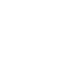
Figure 1. Stress-strain curves for fracture of a <110> Σ3(-1 1 1) Fe symmetric tilt grain boundary. The x, y, and z principle stresses are plotted in red, blue, and green, respectively.
Visualization
The simulation can be visualized in AtomEye. To do so, find the name of the first cfg file (Fe_110_sig3_224.cfg, in this case) that results from the simulation and type "~/A Fe_110_sig3_225.cfg" in a UNIX environment, where "~/A" is the location of the AtomEye file. Alt+0 will color the atoms according to pyy. Use insert and delete to scroll through the images to see the fracture.
Figure 2. Movie showing the fracture of a Fe <110> sigma 3 symmetric tilt grain boundary. Atoms are colored by pyy.
Acknowledgements
The authors would like to acknowledge funding for this work through the Department of Energy.
References
- ↑ S. Plimpton, "Fast Parallel Algorithms for Short-Range Molecular Dynamics," J. Comp. Phys., 117, 1-19 (1995).
- ↑ J. Li, "AtomEye: an efficient atomistic configuration viewer," Modelling Simul. Mater. Sci. Eng. 11 (2003) 173.
- ↑ D.J. Hepburn and G.J. Ackland, "Metallic-covalent interatomic potential for carbon in iron," Phys. Rev. B 78, 165115 (2008).