
Integrated Computational Materials Engineering (ICME)
FeCrHe
Abstract
This is tutorial for K-12 students. This involves the analysis of a relevant research problem in nuclear materials - the segregation of chromium (Cr) and helium (He) to grain boundaries in iron (Fe). This project will introduce a student to using spreadsheet tools to extract information about this important reaction in nuclear energy applications. This is part of a program at Pacific Northwest National Laboratory designed to get high school students involved with STEM-related projects.
Author(s): Mark A. Tschopp, Fei Gao (PNNL), Joanna Sun (student, PNNL)
Background
Here are some questions that may be needed to understand what we are doing in this example.- How does radiation damage materials? Here is a link to Radiation Material Science that gives a relatively good basic explanation of how radiation affects materials.
- What is a point defect? Here is a link to find out about point defects.
- What is a vacancy? It is a type of point defect. Here is a link to find out about a vacancy defect.
- What is an interstitial atom? This is another type of point defect in a material. Here is a link to find out about interstitial defects. This is not used in the present example.
- How are atoms arranged in a metal? Here is a link to find out about crystal structures. In this example, iron (Fe) is a body-centered cubic structure.
- What is a grain boundary? Here is a link to find out about grain boundaries. Grain boundaries join two perfect lattices of different orientations.
- What is segregation? Here is a link to find out about segregation to grain boundaries.
- Why Chromium in Iron? Here is a link to find out about Chromium steels, otherwise known as stainless steels. These are commonly used in the nuclear industry for their corrosion resistance.
Grain Boundary Structure
Viewing the grain boundary structure in Excel
The grain boundary file can be found File:Fe gb 100STGB1 min.data. This file has the following format:
# Minimum Energy GB Structure for LAMMPS

382 atoms
1 atom types
0.000000 6.384740 xlo xhi
-122.293999 122.293999 ylo yhi
0.000000 2.855340 zlo zhi

Atoms

1 1 4.491620 -121.071999 1.713210
2 1 0.105218 -121.735001 0.285542
3 1 0.632080 -119.806999 1.713220
4 1 2.491310 -120.707001 0.285543
5 1 3.150830 -118.677002 1.713220
...
Hints: Copy the file to a directory. How do you load it into Excel so that each number is in a separate cell? When you plot in Excel, how do you make sure that the coordinates aren't distorted (i.e., the spacing in x shouldn't be greater than that in y)? Can you zoom into the grain boundary and see the structure? How is this different from the single crystal lattice? There are two planes in the z-direction - can you plot these as black and white atoms? What are the steps to do this?
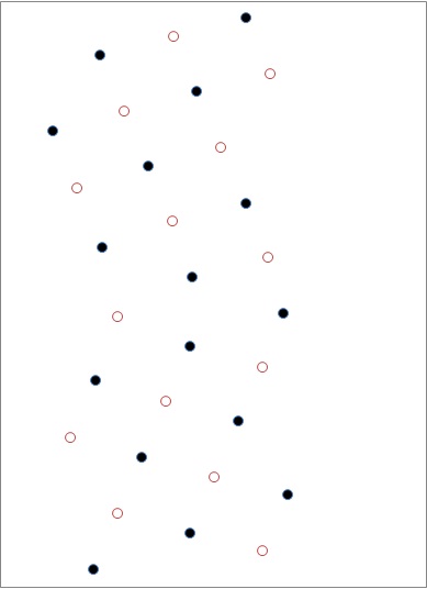
Grain boundary structure. Image of the grain boundary structure, where the white and black atoms represent atoms on different planes into the page.
Steps (How to do this):
Viewing the Grain Boundary Structure (2D) Directions- Open Excel 2010.
- Under the tab “Data”, click “From Web” to import the data directly.
- Go to this site and open the grain boundary file. Select the table of values, and click “Import”. Click “Ok”.
- Select all of the xyz coordinates and under the “Data” tab, click “Text to Columns”.
- The data is Delimited. Make sure “space” is the delimiter and click “Finish”.
- Now the coordinates are separated into columns. Delete column B (the repeated 1’s).
- There are two z values: 0.2854 and 1.7132. Reorganize the coordinates so that you have two columns of xy values with the z value of 0.2854 and two more columns of xy values with the z value 1.7132 adjacent to them. The z values won’t be included in the scatterplot so they can be deleted.
- Select the four columns of coordinates and under the “Insert” tab, click “Scatter” to insert a 2D scatterplot.
- Delete Series 3 by clicking on the Series 3 points and pressing backspace.
- Make Series 1 the first two columns of the data table and Series 2 the last two columns of the data table (Highlight the data points and then drag the corresponding boxes that appear in the table).
- Select the Series 1 points and under the “Format” tab, open the “Format Shape” dialog box and under “Marker Options”, change the marker type to “Built In”. Change the marker type to circles. Under “Marker Fill”, click “Solid Fill” and make the color black. Do the same for Series 2 to change the markers to white circles.
- Double-click on the y-axis to open the Format Axis dialog box. Change the minimum and maximum to fixed values of -10.0 and 10.0, respectively
- Double-click on the x-axis to open the Format Axis dialog box. Change the maximum to the fixed value of 10.0.
- The graph legend, gridlines, and axes can be removed by going under the “Layout” tab and under each, selecting “Do not display”.
Viewing with OVITO
Rather than writing a program to convert from this format to an OVITO format, can you make a new sheet in Excel and rearrange the information from the first file to match the OVITO cfg format. Now you can download OVITO and visualize this information there! A cfg file has the following format:
ITEM: TIMESTEP
0
ITEM: NUMBER OF ATOMS
382
ITEM: BOX BOUNDS
0.000000 6.384740
-122.293999 122.293999
0.000000 2.855340
ITEM: ATOMS id type xs ys zs
4   1 0.000170336 0.0496471 0.0501861
8   1 0.099786    0.0498953 0.0508957
43  1 0.0500606   0.0996001 0.0488291
45  1 0.100489    0.0997987 0.0007703
202 1 0.0499904   0.0502952 0.0993613
...
Hints: Create a new spreadsheet in Excel. Can you identify the different components from the previous file and match them with the elements in this file? Explain. Notice that the coordinates (xs, ys, zs) are scaled coordinates (this is what the s in xs stands for) - this means that the original coordinates need to be rescaled so that all the values fit between 0 and 1 (they won't agree with those in the text box above - I just chose those from another file). Now, you can save this sheet as a text file to load into OVITO. How do you open and view this in OVITO? How do I make the same black and white plot as in the above example in OVITO?
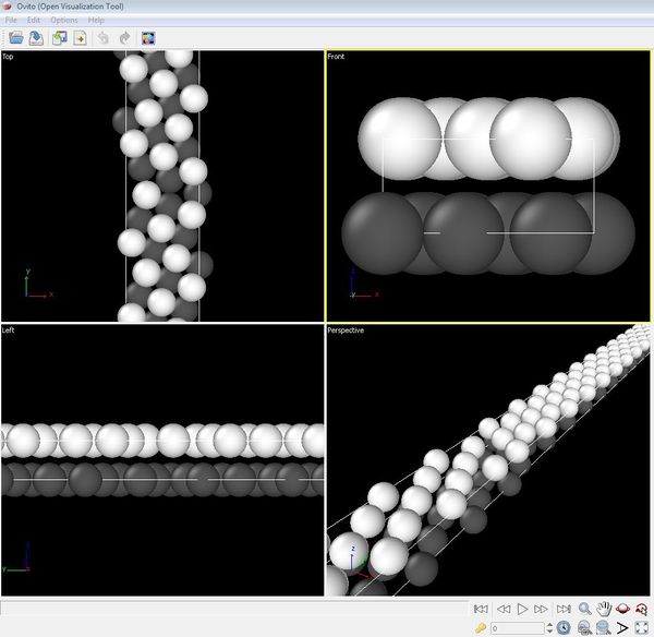
Grain boundary structure in OVITO. Image of the same grain boundary structure as visualized using the atomistic visualization tool OVITO.
Steps (How to do this):
Viewing with OVITO Directions- Open a new spreadsheet in Excel of the atom data.
- The coordinates must be scaled to fit between 0 and 1. Somewhere on the sheet, use the MAX and MIN formulas to find the maximum and minimum values for the x coordinates. Do the same for the y and z coordinates.
- Use a calculator or a function to find the value of (max – min) for x, y, and z.
- You will be using the formula =(point–min)/(max-min). In the next empty adjacent column to the data, type the formula, entering the first x value by clicking on its cell (C10 for example) and filling in the constants you just found for the max and min. Enter the constant you found for (max – min).
- Press Enter and the scaled value for the first x point should appear.
- Highlight this cell, find the black + in the lower right-hand corner, and click and drag the box all the way down the column until the 382nd atom. Now all of the remaining x coordinates should have the formula applied and be scaled.
- Repeat steps 4-6 for the y and z columns of data. Check to see that all of the data points fall in between 0 and 1, inclusively.
- Begin a new sheet. Type the heading information in the format as indicated above.
- Copy all of the newly scaled coordinates from the first sheet and paste them into the second one, making sure to use the paste function “Values”. The format of the data should follow the file example given above.
- Some values in the z column use scientific notation, but we want them in decimal form. Select the column, right click and select “Format Cells”. Under the “Number” tab, select “Number” and have it display 8 or so decimal points.
- The data is now ready to be viewed in OVITO. Save this Excel file.
- Open Notepad. Copy the completed sheet of data and paste it into the new Notepad file.
- Save this text file.
- Open OVITO. Under the “File” tab, click “Import Data”. Choose the text file and under the pull-down menu select “LAMMPS Text Dump File”. Click “Import”.
- The dialog box “LAMMPS Dump File Import Settings” will pop up. The file contains a single snapshot. The five data columns “id, type, xs, ys, and zs” should be in the table. Choose data type “Integer” for id and type and “Float” for xs, ys, and zs. Choose data channel “Atom Index” for id and “Atom Type” for type. Choose “Position” for xs, ys, and zs.
- Click “Ok”. The grain boundary structure should be visualized in OVITO.
For more details on using OVITO, use the user manual as posted on their main website.
Analyzing Cr and He Segregation to the Grain Boundary
Cr-V Formation Energies
In this first example, we are going to look at the Cr-V system. The Cr stands for Chromium and the V stands for vacancy - in essence, we are choosing a site with a particular Fe atom, we are removing this atom to create a vacancy, and then we are replacing this atom with a Cr atom. The formation energy is the energy associated with taking a Cr atom from its perfect state and substituting it into the Fe lattice or grain boundary. I have already ran all the calculations.
First, we are going to plot these results in Excel. Attached are the energies for the grain boundary with a Cr atom replacing an Fe atom at a particular site (File:Fe gb 100STGB1 min.Cr.txt). The format is below. Notice that the ID starts at 169 - this is because I only ran simulations for those atoms that were within 15 Angstoms (15 x 10-10 meters... really small!) of the grain boundary (the y-coordinates run from -15 to 15). The E_sub is the formation energy of substituting a Cr atom for an Fe atom (in electron volts, eV) - in a perfect single crystal, this energy is -0.287 eV.
ID      x            y            z           E_sub
169     1.874770   -13.902000     1.713240    -0.286553
170     3.791050   -14.539400     0.285573    -0.287263
Hints: How does this change as a function of distance from the grain boundary? Plot energies versus the y-coordinate. Is it the same on either side of the grain boundary? Does what plane the atom lies on in the z-direction affect the energy (it shouldn't, plot anyway)? Is there a way to plot a 3D plot in Excel where you can look at the x and y coordinates along with the energy? What do you see? (This might be cooler later with more complex grain boundary structures).
Steps (How to do this):- Open Excel. Import the data using methods used previously.
- Again, use the “Text to Columns” function to separate the data columns.
- Use the scatterplot graph function to view the y points plotted against the formation energies.
- In a new sheet, scale the x,y,z, and Evf_Cr values using the method discussed above.
Now we are going to visualize this in OVITO. Again, we have to modify our spreadsheet to add the formation energy of Cr (Evf_Cr) in every site as well (i.e., E_sub above). Notice any trends?
The OVITO file should look like this:
ITEM: TIMESTEP
0
ITEM: NUMBER OF ATOMS
382
ITEM: BOX BOUNDS
0.000000 6.384740
-122.293999 122.293999
0.000000 2.855340
ITEM: ATOMS id type xs ys zs Evf_Cr
4   1 0.000170336 0.0496471 0.0501861   -0.286553
8   1 0.099786    0.0498953 0.0508957   -0.284323
43  1 0.0500606   0.0996001 0.0488291   -0.283522
45  1 0.100489    0.0997987 0.000770305 -0.287666
202 1 0.0499904   0.0502952 0.0993613   -0.286553
...
The addition steps:
- Reorganize the data for viewing in OVITO using the format and methods discussed above. Use the max and mins of the data for the box bounds. This set of data only has 46 atoms. Renumber the atoms from 1-46.
- Transfer the data to a Notepad text file. Import the data into OVITO. This time, the “LAMMPS Dump File Import Settings” box needs to include the Evf_Cr row in addition to id, type, xs, ys, and zs. Click “Automatically Assign” and the data type (Float) and channel (Evf_Cr) should be assigned.
- Click “Ok” and the new grain boundary will be visualized.
- We want the color of each atom to correspond to its Cr-V energy. Under the “Modifier List” menu, select “Color Coding”. Under “Data Channel”, select “Evf_Cr” and click “Adjust range”.
Cr-V interacting with V Formation Energies
This case is a little different. For each site, a Cr atom is substituting an Fe atom (Cr-V, per above). However, then we are identifying a neighboring atom and removing it to create a vacancy. Now the energy is calculated. Since each atom may have between 4-8 neighbors, there are multiple possible combinations of Cr-V interacting with a vacancy - so each combination required a different calculation. Attached are the energies for this situation where each line represents a different simulation (File:Fe gb 100STGB1 min.CrV-V.txt). The format is given below:
Cr_ID Cr_x Cr_y Cr_z Vac_ID Vac_x Vac_y Vac_z E_total
169 1.874770 -13.902000 1.713240 167 1.237690 -15.817200 0.285576 -22950.771540
170 3.791050 -14.539400 0.285573 165 3.153750 -16.455299 1.713250 -22950.770900
171 4.428600 -12.623300 1.713240 170 3.791050 -14.539400 0.285573 -22950.770620
...
169 1.874770 -13.902000 1.713240 170 3.791050 -14.539400 0.285573 -22950.769480
170 3.791050 -14.539400 0.285573 168 5.706740 -15.178100 1.713250 -22950.770860
171 4.428600 -12.623300 1.713240 172 6.344010 -13.262200 0.285570 -22950.771190
...
Similar to earlier, the atom ID of the Cr atom is given along with the x, y, and z coordinates of the Cr-V location. Also, the atom ID of the Fe atom that was removed is in column 5 along with the x, y, and z coordinates of the vacancy. The total energy is given. The formation energy will need to be calculated. In order to do this, the energy of the original grain boundary without any defects needs to be calculated. Here is the file from the atomistic code that gives that energy (File:Fe gb 100STGB1 min.Gb0.txt and search for 'lattice energy').
More involved project:- Calculate the formation energy for every defect (same formula for all)
- How does this change as a function of position?
- Does the formation energy change for a single Cr-V site for the different neighbors? (Probably not as much in the bulk lattice, but at the grain boundary it should) How does the maximum, minimum, and range (max-min) of the formation energies for each site change as a function of position?
- How can we view this in OVITO? Can we put together a master OVITO file with Cr-V energies (above) along with CrV-V energies from this example?
- If you were to draw a vector from every Cr-V to every V, is there some relationship between the energies and the vectors? That is, for y-coordinates above 0, if the vector points towards the grain boundary (at y=0), does this result in lower formation energies?
- Overall, is there much difference between the CrV and the CrV-V cases?
- Calculate the binding energy between the vacancy and the Cr-V defect (need vacancy formation energy). How does this change as a function of position? Note that the binding energy between a vacancy and the Cr-V defect in the bulk lattice is small.