Abstract

This example shows how to plot a journal quality plot in MATLAB. This is my tried and true methodology for producing eps and pdf figures in MATLAB!

Author(s): Mark A. Tschopp

MATLAB Script

This shows a plot for binding energy as a function of distance for point defects near a grain boundary. The plot can be saved as a MATLAB figure after it appears. Additionally, the exportfig command, which refers to a script that can be downloaded at the MATLAB Central File website, exports the plot to a jpeg, tiff, or eps file.

mean1 = [0.448 0.475 0.411 0.257 0.147 0.071 0.032 0.013 0.008 0.004 0.002 0.002 0.001 0.001 0.001 -0.000];
std1 = [0.253 0.218 0.197 0.147 0.095 0.062 0.036 0.019 0.017 0.009 0.008 0.007 0.007 0.007 0.005 0.003];
mean2 = [2.194 2.204 2.141 1.900 1.577 1.131 0.665 0.312 0.134 0.051 0.025 0.014 0.010 0.008 0.005 -0.001];
std2 = [0.617 0.573 0.587 0.716 0.768 0.721 0.556 0.372 0.245 0.167 0.141 0.126 0.125 0.122 0.132 0.147];

errorbar(0:15,mean1,std1,'-sr','LineWidth',2,'MarkerFaceColor','w','MarkerEdgeColor','r')
hold on
errorbar(0:15,mean2,std2,'-ob','LineWidth',2,'MarkerFaceColor','b','MarkerEdgeColor','b')

axis([0 15 0 3.25])
axis square
%set(gca,'Box','off')

xlabel('Distance from Grain Boundary (Angstroms)', 'FontSize',30, 'FontName','Times', 'FontWeight','b');
ylabel({'Binding Energy (eV)'}, 'FontSize',30, 'FontName','Times', 'FontWeight','b');
set(gca, 'FontSize',24, 'FontName','Times', 'LineWidth',2);
set(get(gca,'Children'),'MarkerSize',10)
set(gcf,'Position',[1 1 round(1200) round(1200)])
legend('Mean Vacancy Binding Energy', 'Mean Interstitial Binding Energy','Location',[0.6 0.70 0.1 0.1])
legend('boxoff')

annotation('textbox',[0.67 0.87 0.00 0.00],'String','Binding Energy Plot', 'FontName','times','FontSize',30,'fontweight','b','LineWidth',1,'Color','k', 'HorizontalAlignment', 'center','BackgroundColor','k','FitBoxToText','on')
annotation('textbox',[0.68 0.88 0.00 0.00],'String','Binding Energy Plot', 'FontName','times','FontSize',30,'fontweight','b','LineWidth',1,'Color','r', 'HorizontalAlignment', 'center','BackgroundColor','w','FitBoxToText','on')

exportfig(gcf,'plot_binding.jpg','Format','jpg','Color','rgb','Resolution',300)
exportfig(gcf,'plot_binding.tif','Format','tiff','Color','rgb','Resolution',300)
opts = struct('Format','eps','Color','rgb');
exportfig(gcf,'plot_binding.eps',opts)
saveas(gcf,'plot_binding.fig','fig')
close(1)

The eps file can be directly used for journal papers or converted to pdf format, depending on preference. There is a MATLAB utility program eps2pdf to convert directly using MATLAB from the command line or within a script. OR you can use UNIX's eps2pdf command to convert to pdf. These formats are often useful for LaTEX and pdfLaTEX.

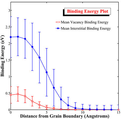
Figure 1. Binding energy for point defects.