Abstract

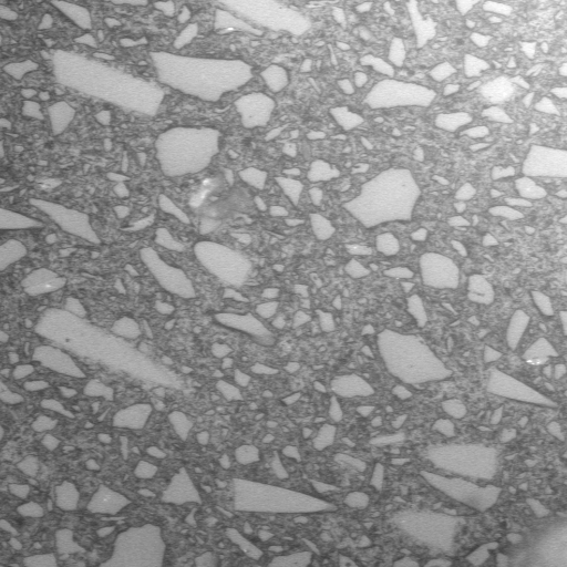
This is an introduction to image processing with MATLAB using the basic example shown below. In this tutorial we are going to segment the particles in this image.

Author(s): Mark A. Tschopp

Corresponding Author: Mark Tschopp

Tutorial

1. Download the File:SAND.TIF image.
2. Open MATLAB with Image Processing Toolbox
3. First, let's open the image. Start with the uigetfile command which opens a pop-up window with all the files of the type '*.tif'. Select the image that you want to process, in this case 'SAND.TIF'. The imread command will read in the image. Notice that after executing the imread command, the variable I shows up in the variable stack window as a 512x512 matrix with type uint8 (i.e., an 8-bit image). The type uint8 means that the pixels have integer values in the range of 0 to 255. This means that if 255 is added (or subtracted) to the image (i.e., I = I + 255;), all the pixels will have a value of 255 (or 0 in the case of subtraction of 255).



fname = uigetfile('*.tif');
I = imread(fname);



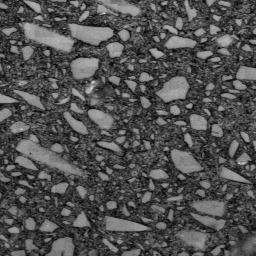
4. View the image using the imshow command. The [] command will use the minimum and maximum pixel values to give good contrast within the image (if necessary). Using imshow(I) will often work as well.



imshow(I,[])



5. View a histogram of the pixel intensities using the imhist command. Notice that there is not a lot of contrast between the particles and the matrix (as a result of the gradual change in intensity from the lower left to upper right).



imhist(I)



6. Method 1 - Try to segment the image using an intensity threshold of 170 and then show the new binary image, J1. The first line here identifies all pixels that have an intensity greater than 170 as 1 (true) and all intensities below or equal to 170 as a 0 (false). Notice that J1 is the same size and I and that J1 is a logical matrix (meaning that it can only have 0's and 1's). This method does a poor job of segmenting the image because of the intensity change over the background.



J1 = I > 170;
imshow(J1,[])



7. Method 2 - Try to segment the image using an automated global intensity threshold technique (Otsu's method^[1]). The graythresh function uses Otsu's method, which chooses the threshold to minimize the intraclass variance of the black and white pixels. The pixel line gives the intensity threshold defined by this function and im2bw segments the image according to the threshold defined via the graythresh command. Then show the new binary image, J2. This still doesn't work, because there isn't enough separation between the two histograms.



level = graythresh(I);
pixel = level * 255;
J2 = im2bw(I,level);
imshow(J2)



8. Method 3 - First, apply a filter to find the darkest pixel in each region. You can use either the ordfilt2 command or the imerode command to find the darkest pixel in a region of size 'nsize' around each pixel. Then show this image using imshow.



nsize = 40; 
I_background = ordfilt2(I,1,true(nsize),'symmetric');
I_background = imerode(I,strel('square',nsize));
imshow(I_background,[])



9. Now we want to subtract this from the initial image I. This image processing levels the background intensity of the image. Remember that our image I is stored as uint8, though, so we need to transform it to a double precision matrix before subtracting. The imshow command will show the new leveled image.



I_leveled = double(I) - double(I_background);
imshow(I_leveled,[])






10. Now we tranform it back to a uint8 image by rescaling the values to integers between 0 and 255. We are going to store this as our new and improved image, I2. Let's also look at the image histogram. Notice how the two distributions have separated by leveling the image.



I_leveled = uint8((I_leveled - min(I_leveled(:)))/(max(I_leveled(:)) - min(I_leveled(:))) * 255);
imhist(I_leveled)



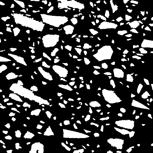
11. Now we are just going to manually segment the image using an intensity of 120.



manual_threshold = 120;
J3 = I_leveled > manual_threshold;
imshow(J3,[])



12. Let's get rid of everything below a certain size using the bwareaopen command and then show the new image.



BW2 = bwareaopen(BW,10)
imshow(BW2)




or we could have used another approach

BW = J3;
CC = bwconncomp(BW);
L = labelmatrix(CC);
stats  = regionprops(L);
area = [stats.Area];
size_thresh = 10;
idx = find(area > size_thresh);
BW2 = ismember(L, idx);
imshow(BW2)



13. Let's fill in the holes



BW3 = imfill(BW2,'holes');
imshow(BW3)



14. I tried something a little different here, just for fun. So, first, I dilated (expanded) the white regions (particles) using a square 5x5 region. Then I used Otsu's technique to find a suitable threshold for ONLY the pixel intensities within the dilated white regions. I used this threshold to segment the particles and deleted any segmented objects in the black regions by setting their intensity equal to 0. I then filled in the holes and deleted any objects smaller than 30 pixels. Last I show the final image. Do you see that...?



BW_trial = imdilate(BW3,strel('square',5));
imshow(BW_trial)
level = graythresh(I_leveled(BW_trial));
pixel = level * 255;
BW4 = im2bw(I_leveled,level);
BW4(~BW_trial) = 0;
BW4 = imfill(BW4,'holes');
BW4 = bwareaopen(BW4,30);
imshow(BW4,[])






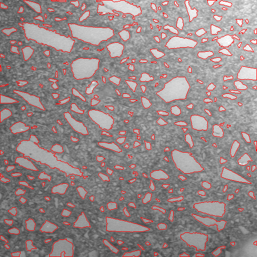
15. Now let's show on the original image. First, we create a binary image that contains only the pixels on the perimeter of our particles using the bwperim function. Then, we are generating a new RGB image I2 with 3 channels - I2(:,:,1) RED, I2(:,:,2) GREEN, I2(:,:,3) BLUE. We are setting only the perimeter pixels to red by changing their intensities to 255 for the red channel and 0 for the green and blue channels. Voila!



BW5 = bwperim(BW4);
imshow(BW5,[])
I2 = I; I2(BW5) = 255;
I_RGB = I2;
I2 = I; I2(BW5) = 0;
I_RGB(:,:,2) = I2;
I2 = I; I2(BW5) = 0;
I_RGB(:,:,3) = I2;
imshow(I_RGB,[])






16. Go ahead and save the images using the imwrite command



imwrite(I_RGB,'image_RGB.tif','tif')
imwrite(BW4,'image_binary.tif','tif')
imwrite(I_leveled,'image_leveled.tif','tif')

References

1. ↑ Otsu, N., "A Threshold Selection Method from Gray-Level Histograms," IEEE Transactions on Systems, Man, and Cybernetics, Vol. 9, No. 1, 1979, pp. 62-66.