Help

Show information regarding the application, or reset the application.

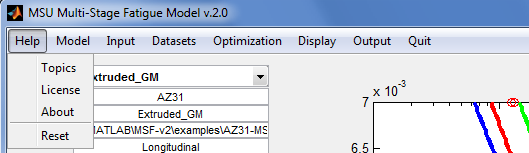
• Topics - Display the help file on a browser.


• License - Display the license file on a browser.


• About - Display the current version of the tool and the contact information of the developer/maintainer.


• Reset - Re-initialize the tool in case something goes wrong. Data and properties loaded, as well as revised settings, will be lost if not written to files (see Output).

Model

Select which MSF model to use.

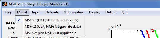
• MSF v1 (NCF; strain-life data only) – Use MSF version 1, for strain life data. Model has incubation and small crack parameters.


• (IN DEVELOPMENT; DO NOT USE) MSF v2 (CLP, NCF; fatigue-life data) – Use MSF version 2, to model crack length propagation and number of cycles to fatigue. Model has incubation, small crack, and long crack parameters. For strain-life, stress-life, and some other types of fatigue life data.


• (IN DEVELOPMENT; DO NOT USE) MSF v2; plot MSF v1 if applicable – Use MSF version 2, and also plot the MSF version 1 model if applicable.

Input

Load a file into the application.

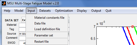
• Material constants file - Open a file selection dialog for the name of a material properties file to be retrieved into the application. A material constants file is created from the displayed parameters through the menu item Output | Material constants file. See File:MSFv2 file constants.txt for an example.


• Data file - Open a file selection dialog for the name of a fatigue life dataset to be retrieved into the application. This is a text file containing measurements from a fatigue life experiment, loading information, material constants, and microstructure information. See File:MSFv2 file data.txt for an example.


• Load definiton file - Open a file selection dialog for the name of a load definition file to be retrieved into the application. (YHAMMI to describe what is a load definition file.)


• Parameter set - Open a file selection dialog for the name of a “properties and constraints” file to be retrieved into the application. This is a text file containing lines with the format "name=value fix min max", where name is a fitted constant in the MSF model, fix is 0 or 1 to indicate that the value is to be fixed during optimization, and [min, max] is the range of permissible values for the constant if fix=0. This file may be created through the menu item Output | Parameters set from the parameters displayed in the GUI. See File:MSFv2 file constraints.txt for an example.


• Restart file - Open a file selection dialog for the name of a “restart” file to be retrieved into the application. A restart file is a record of the state of a previous model fitting session. This file is created by the menu item Output | Restart file during that session. Loading the restart file effectively resumes the previous session.

Datasets

Temporarily exclude datasets from the model fitting process, or permanently remove datasets from memory.

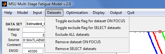
• Toggle exclude flag for dataset ON FOCUS – This menu item toggles the “exclude” flag for the dataset currently on focus (i.e., the dataset displayed on the left panel of the GUI). The exclude flag for a dataset determines whether or not the dataset will be plotted or used during model fitting. If the value of the flag is true, the dataset is excluded and “(excl)” is appended to its tag.


• Toggle exclude flag for SELECT datasets – Open a dialog to select datasets, then toggle the exclude flags for those datasets.


• Exclude ALL datasets - Set the exclude flags of all datasets to true.


• Remove dataset ON FOCUS - Remove the dataset currently on focus from memory.


• Remove SELECT datasets - Open a dialog to select datasets, then remove the datasets from memory.

Optimization

Select the optimization method and set its options.

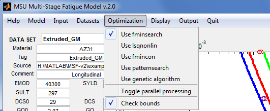
• Use fminsearch - Set options for MATLAB's fminsearch(), then use it as the optimization routine. This routine attempts to find a minimum of a scalar function of several variables, starting at an initial estimate, using a derivative-free simplex search method. This method may find a solution outside of the specified parameter ranges.


• Use lsqnonlin - Set options for MATLAB's lsqnonlin(), then use it as the optimization routine. This routine solves nonlinear least-squares curve fitting problems. The default algorithm is a subspace trust-region method and is based on the interior-reflective Newton method.


• Use fmincon - Set options for MATLAB's fmincon(), then use it as the optimization routine. The routine attempts to find a constrained minimum of a scalar function of several variables starting at an initial estimate. The technique is generally referred to as constrained nonlinear optimization or nonlinear programming.


• Use patternsearch - Set options for MATLAB's patternsearch(), then use it as the optimization routine. This routine finds the minimum of a function using pattern search.


• Use genetic algorithm - Set options for MATLAB's ga(), then use it as the optimization routine. This routine finds the minimum of a function using genetic algorithm.


• Toggle parallel processing - Enable/disable parallel processing in the following optimization routines: lsqnonlin(), fmincon(), patternsearch(), and ga().Parallel processing is available when the application is running under MATLAB on a multi-core machine.


• Check parameter bounds - Before running an optimization, check that the initial parameters are withing their specified [min, max] ranges.

Display

Modify the appearance of plots and the GUI.

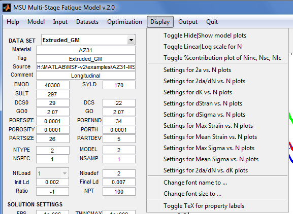
• Toggle Hide or Show model plots - Enable or disable calculation of the MSF model points from the properties currently on display. When the application starts, there may not be sufficient information to evaluate the model; hence, the initial setting is to hide the model plots.


• Toggle Linear or Log scale for N - Use linear scale or logarithmic scale for the horizontal axis.


• Toggle %contribution plot of Ninc, Nsc, Nlc – Enable or disable generation of stacked bar plots showing the contributions (in %) of incubation cycles, small crack cycles, and long crack cycles to the total number of cycles.


• Settings for TYPE plots, where TYPE is one of 2a vs. N, 2da/dN vs. N, dK vs. N, dStran vs. N, dSigma vs. N, Max Strain vs. N, Mean Strain vs. N, Max Sigma vs. N, Mean Sigma vs. N, 2da/dN vs. dK - These menu items open a dialog to modify the appearance of the plot area. The following may be set in the dialog: scaling of the x-axis; labels and lower/upper limits for the x- and y- axes; thickness of plot lines; size of plot markers; hide/show grid lines; plot title; legend position; and, components (incubation, small crack, long crack, total cycles) of the model to plot.


• Change font name to ... – Open a dialog to select the font style. The fonts in the plot area will be changed when the GUI is updated. The platform on which the application is executing determines the font styles that are available.


• Toggle TeX for property labels – Toggle between ordinary text or TeX math symbols for the property labels.

Output

Create output files.

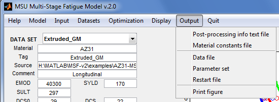
• Post-processing info textfile - Open an input dialog for the name of a “post-processing information” file to be created by the application. This is a text file of comma separated values, and is suitable for import into a spreadsheet program like MS Excel. This file contains the model parameters currently on display, the fatigue life datasets used in fitting the parameters, and the model points. Such post-processing information is typically used to produce publication-quality plots of the model points, or for "cut-and-paste" into a report. The MSF2.txt extension is automatically appended to the filename.


• Material constants file - Open an input dialog for the name of a material constants file to be created from the parameters currently on display. Descriptions of the constants are included. The extension MSF2.props is automatically appended to the filename. This file may be loaded into the application in the future using the menu item Input | Material constants file, or used as input to another program, or for "cut-and-paste" of the material constants into a report. See File:MSFv2 file constants.txt for an example.


• Data file - Open a dialog to select the data set for which a data file will be created by the application. This will be a text file containing material identifier, material constants, microstructure information, loading information, and experimental data. Descriptions of the information are included. The extension MSF2.data is automatically appended to the filename. This menu item is useful for creating templates of data files from a restart file. See File:MSFv2 file data.txt for an example.


• Parameter set - Open an input dialog for the name of a “properties and constraints” file to be created by the application from the parameter set currently displayed in the GUI. Descriptions of the properties are included. This is a text file containing lines with the format "name=value fix min max", where name is a fitted constant in the model, fix is 0 or 1 to indicate that the value is to be fixed during optimization, and [min, max] is the range of permissible values for the constant if fix=0. The extension MSF2.params is automatically appended to the filename. This file may be loaded into the application in the future using the menu item Input | Parameters set. This menu item is useful for creating a template for an input parameter set from a restart file or from the parameter set currently on display in the GUI. See File:MSFv2 file constraints.txt for an example.


• Restart file - Open an input dialog for the name of a “restart” file to be created by the application. This is a binary file that records the state of the model fitting session (the datasets loaded, the parameter sets attempted, and the solution settings). The extension MSF2_restart.mat is automatically appended to the filename. This file may be loaded at some future time using the menu item Input | Restart file to resumes the session. This feature is useful if the user gets tired and wishes to continue the fitting session after getting some sleep.


• Print figure - Open a “print preview” of the application window. A snapshot of the window can then be sent directly to a printer.

Quit

Exit or reset the application.

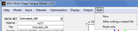
• Now - Turn off parallel processing if previously enabled, then exit the application.


• After writing a restart file – Output a restart file (automatically named “LAST_SESSION-MSF2_restart.mat”), turn off parallel processing if previously enabled, then exit the application.


• Reset only (same as Help | Reset) – Re-initialize the application in case something goes wrong. Data and properties previously loaded into the application, as well as revised settings, will be lost.

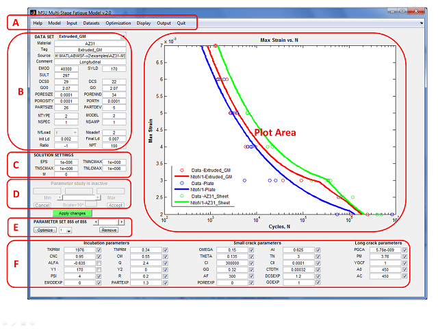
Dataset Controls

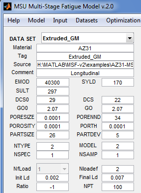
• DATA SET - Popup menu to select the dataset whose elements will be displayed. If none is selected, the rest of the data set controls will be filled with blanks; otherwise, the controls will be updated with values from the selected dataset.


• Material - Text; identifier for material


• Tag - Text; to differentiate data sets


• Source - Text; the source of data set


• Comment - Text; any other comment on data set


• EMOD - Number; Young's modulus [MPa]


• SYLD - Number; Yield stress [MPa]


• SULT - Number; Ultimate Stress [MPa]


• DCS0 - Number; Reference grain size (microns)


• GO0 - Number; Reference grain orientation


• PORESIZE - Number; Pore size


• PORENND - Number; Pore nearest neighbor distance


• POROSITY - Number; Porosity


• PORTH - Number; Porosity threshold


• PARTSIZE - Number; Particle size average


• PARTDEV - Number; Particle size standard deviation


• NTYPE - Type of fatigue loading: 1=Crack length propagation, 2=Fatigue life


• MODEL - 1=Elastic, 2=Plastic


• NSPEC - Number of spectrum fatigue loads (0 for undetermined and crack length limit)


• NfLoad - Number of applied fatigue loads


• [Nloadef, Init Ld, Final Ld, Ratio, NPT] – Fatigue loading definition

Changes to values in edit boxes take effect after selecting the Apply Changes push button. The plot of the model for the dataset will be updated automatically.

Solution Settings

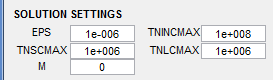
• EPS - Convergence criterion for DSIGMA


• TNINCMAX - Maximum cycles for incubation


• TNSCMAX - Maximum cycles for small crack


• TNLMAX - Maximum cycles for long crack


• M - Comment check code (debugging flag in MSF code; must be 0 to prevent code from generating debugging messages)

Changes to values in edit boxes take effect after selecting the Apply Changes push button. The model plots will be updated automatically.

Parameter study controls

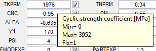
Each model parameter (see Model Parameters) is associated with four interface elements: the current value edit box, a range of permissible values during optimization (not visible), and a fix check box to indicate that the parameter is fixed (not to be changed) during optimization. A description of the parameter and the range are displayed by hovering the pointing device over the current value edit box (TNPRM, for example, in the figure on the right).


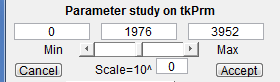
A right-click on the current value edit box of a parameter initiates a parameter study. The Parameter study controls are enabled while all other controls are disabled. The range constraint for the parameter is transferred to the Min and Max edit fields as well as to the slider limits. The current value is transferred to the middle edit box and is used to initially position the slider. Any of these values may be edited directly. Changes will take effect after clicking anywhere in the window outside of the edit boxes.

Operating the parameter study slider decreases or increases the parameter value, depending on where the slider bar is positioned. The model plots are updated automatically with each change of the current value.

If the Min value is close to the Max value, the slider may not work properly due to the resulting low resolution of the slider steps. In this case, setting the scale (Scale=10^ edit box) to a negative integer may restore the expected functionality. Similarly, for a large range of values, setting the scale to a positive integer may prevent huge jumps the parameter value when the slider is operated.

Accept creates a new parameter set from the set currently on focus, with the current value and range constraint for the selected parameter coming from the edit boxes. This also exits the parameter study. Cancel exits the parameter study without any changes to the selected parameter.

Parameter set controls

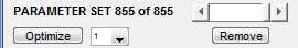
A parameter set is simply the collection of all the parameters. A record of all parameter sets attempted by the user is maintained by the GUI. This record may be navigated by moving the PARAMETER SET slider. The parameter set currently on focus may be discarded by selecting the Remove push button, after which the next available parameter set automatically becomes the focus. A number of parameters may be modified before selecting the Apply changes push button to create a new parameter set. The Optimize button invokes the optimization module to automatically update the parameters that are not fixed.

Tip: A parameter that is set to zero may be respected by the optimizer, and may remain zero even if this is not fixed. For the parameter to participate in fitting, set it initially to a "small" value.

Determining the proper model parameters for a material is a trial and error process, and can be time consuming and tedious. Even if starting with reasonable guesses for initial values, perhaps from a similar material, many interactions with the GUI will be required to arrive at a solution. The best approach is to guide the process with some thoughtful consideration on the influence of the parameters on model.

The GUI discussed here is helpful to make changes in the parameters and see the effect on the response. The optimization routines are available, but should not be relied on. Optimization will produce a mathematically optimal solution, but this may not correspond to the underlying physics. The better use of the optimization is to use guided, human direction of the process, and use optimization on just a few parameters at any one time to improve the solution. Using the optimization feature to produce a solution, allowing the procedure to change many variables at once, will almost certainly lead to a lengthy process without good results.

Fitted parameters

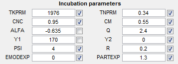
Incubation parameters

• TKPRM - Cyclic strength coefficient [MPa]


• TNPRM - Cyclic strain hardening exponent


• CNC - Constant related to Coffin Manson Law


• CM - Ductility coefficient in Coffin Manson Law


• ALFA - Ductility exponent in Coffin Manson Law


• QQ - Exponent in remote strain to local plastic shear strain


• Y1 - Constant in remote strain to local plastic shear strain


• Y2 - Linear constant in remote strain to local plastic shear


• PSI - Geometric factor in micromechanics study


• R - Exponent in micromechanics study


• EMODEXP - Shape parameter for Young's modulus


• PARTEXP - Shape parameter for particle size

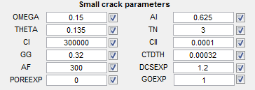
Small crack parameters

• OMEGA - Pore effect coefficient


• AI - Initial crack size contribution


• THETA - Load path dependent and loading combination parameter


• TN - Exponent in Small Crack growth


• CI - LCF constant in small crack growth


• CII - HCF constant in small crack growth


• GG - Crack growth rate constant


• CTDTH - CTD threshold value


• AF - Final crack size length (microns)


• DCSEXP - Crack growth rate constant (G)


• POREEXP - Effect of pore size to local plastic strain


• GOEXP - Grain orientation effects exponent

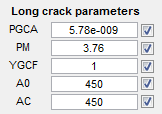
Long crack parameters

• PGCA - Paris Crack Growth Parameter


• PM - Paris Exponent


• YGCF - Geometrical Correction Function


• A0 - Small crack length


• AC - Long crack length (at coalescence)

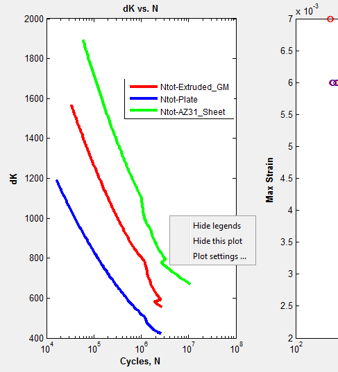
Plot area

If MSF model version 1 is selected as the model to use, strain-life data plots and the corresponding fatigue life model points are displayed on the plot area. With MSF model version 2, the following data and model plots may be displayed: 2a vs. N; 2da/dN vs. N; dK vs. N; dStran vs. N; dSigma vs. N; Max Strain vs. N; Mean Strain vs. N; Max Sigma vs. N; Mean Sigma vs. N; and 2da/dN vs. dK.

The settings for each type of plot (scaling of the x-axis; labels and lower/upper limits for the x- and y- axes; thickness of plot lines; size of plot markers; etc.) may be specified by selecting the menu item Display | Settings for ….

Alternatively, if a plot is currently on display, a right-click on an empty area in the plot activates a context menu which initiates the dialog to specify the plot settings, or to disable the altogether.

Parallelism in MSF

When parallel-enabled (see Optimization | Toggle parallel processing), the manner in which the MSF application utilizes multiple cores depends on the setting of the pop-up menu beside the Optimize button(). This pop-up determines the number of starting solutions when you click Optimize.

IF you specify one starting solution (i.e., "Optimize 1") AND you specify "Use fmincon" or "Use patternsearch" or "Use genetic algorithm" as the optimization method, THEN MSF will use the multiple cores. The starting solution for the optimization are the displayed parameters, and the final solution is whatever the optimization method will find when starting from these parameters. The methods fmincon, patternsearch and genetic algorithm have parallel implementations in MATLAB; hence, the optimization process will benefit from the multiple cores. The methods fminsearch and lsqnonlin DO NOT have parallel implementations (as of MATLAB R2012a), so optimization with these methods will NOT benefit from multiple cores with "Optimize 1" (however, these will still find final solutions).

IF you specify "Optimize N", then MSF will automatically generate a number of starting solutions as follows. Let K be the number of MSF parameters that are NOT fixed (i.e. unchecked in the MSF user interface). The "global" search space for the optimization is the K-dimensional hyper-rectangular region R = [min_1,max_1] * [min_2,max_2] * ... * [min_K,max_K], where [min_i,max_i] is the range for the i-th parameter. MSF will divide each range will into N subintervals so that there will be N^K (N to the power K) hyper-rectangular subregions.

MSF will generate a random starting solution within each subregion, and run an optimization from the random starting point. The optimization will be bounded by the limits of the subregion (except if the method is fminsearch).

The following is a small table for N^K, the number of optimization runs to be performed by MSF. Since one run might take several seconds or a few minutes, the whole process may still require a significant wait even if MSF will perform the runs in parallel.

MSF will collect a number of "locally good" results, along with the limits of the subregions returning such results. When all the N^K searches are complete, you can browse the results and manually decide which are "really good". Not all subregions will produce "good" results; hence, much much less than N^K results will be returned.

N^K	K=2	K=3	K=4	K=5	K=6	K=8	K=10	K=12
N=2	4	8	16	32	64	256	1024	4096
N=3	9	27	81	243	729	6561
N=4	16	64	256	1024	4096
N=5	25	125	625	3125

Thus, "Optimize N" is intended to be used with "small N" and "small K" for semi-automated exploration of the search space, if you have no idea what are "reasonable combinations of limits" for the model parameters.