Overview

DMGfit is an interactive calibration tool for the Mississippi State University Internal State Variable Damage and Plasticity (MSU ISV DMG) model. The model is written in Fortran as an ABAQUS User Material subroutine (UMAT). DMGfit is used to determine 'material constants' which will be used as inputs along with this UMAT to a finite element simulation in ABAQUS.

The current version of the MSU ISV DMG model (55p-v1p1) is specified by 55 constants. Some of these constants, like bulk modulus, shear modulus, and melting temperature, are fixed for a given material and may be obtained from the literature. Other constants, such as average radius of voids, average size of particles, and average grain size, are measured from characterization experiments on samples of the material. The remaining constants are fitted, using DMGfit, from stress-strain data from experiments on the samples.

In the following figure, the upper-left region shows a screenshot of the stand-alone DMGfit, while the upper-right region abstracts an ABAQUS simulation with inputs including the material properties and the UMAT. In the lower part of the figure, the region outlined by red dashes provides high-level descriptions of the model calibration and plotting processes underlying DMGfit.


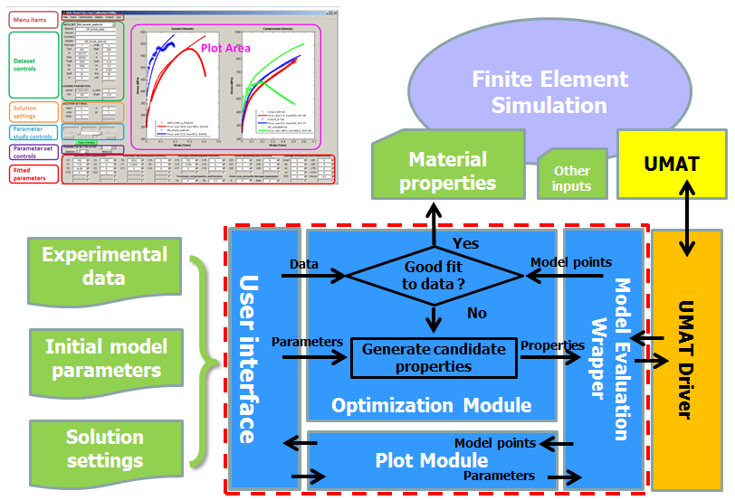
A DMGfit user specifies the experimental data, initial model parameters, and solution settings through the User interface. The Plot Module invokes the model code to calculate the model points from the material parameters currently on display. The model points are plotted alongside the experimental data. Individual parameters may be manually edited on the User interface to change the shape of the model curve. The Optimization Module attempts to automatically find values for a user-specified set of parameters which will generate model points that are "close" to the experimental data.

The Plot and Optimization modules are written in MATLAB. The Model Evaluation Wrapper (MATLAB) and the UMAT Driver (Fortran) serve as bridges between the Plot and Optimization modules and the model UMAT. The User interface for the stand-alone version of DMGfit is written in MATLAB; for the online version of DMGfit, the User interface is a Web page.

The online version of DMGfit (for MSU ISV DMG version 1.0, or 54p-v1p0) is NO LONGER available.

A zipped executable for the stand-alone version of DMGfit (for MSU ISV DMG version 55p-v1p1) on 64-bit Windows 7 PCs without MATLAB is File:DMG-development.zip. This was compiled using MATLAB R2014b and Intel Visual Fortran 12.0 (with Microsoft Visual C++ 2010 linker). Unzip, then run MyAppInstaller_web.exe. The default installation directory is C:\Program Files\DMG_development. The MATLAB Compiler Runtime (v84) will be downloaded and installed automatically if not yet present in the local machine. After installation, run DMG_development.exe in C:\Program Files\DMG_development\application. As a test, load one of the restart files included with the executable.

A tutorial is File:DMGfit-Tutorial.zip. Similarly, a video can be found here.

The stand-alone version is parallel-enabled to take advantage of up to 12 cores on multi-core PCs and workstations.

DMGfit is also described in Chapter 6 of Applications from Engineering with MATLAB Concepts - Case Studies in Using MATLAB to Build Model Calibration Tools for Multiscale Modeling

The Graphical User Interface

A snapshot of the DMGfit Graphical User Interface (GUI) in operation, annotated to highlight the logical groupings of the GUI controls, is shown by the figure below.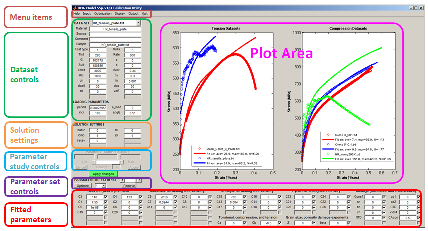


Menu items - input/output operations, optimization options, and plot appearance settings.

Dataset controls - describes the experimental stress-strain data measured from a sample of the material under consideration. These controls include damage model constants that are fixed, from the literature or measured from the sample represented by the data set, as well as loading parameters required by the UMAT Driver to model the experiment.

Solution settings - additional parameters required by the UMAT Driver.

Single Parameter study controls - activated by a right-click on a fitted parameter, to investigate the solitary effect of the parameter on the model.

The Apply changes button - commits changes to values in edit boxes (dataset items, loading parameters, solution settings, fitted parameters) or check boxes in the GUI.

Parameter set controls - operations that apply to the current set of fitted parameters.

Fitted parameters - model parameters to be calibrated.

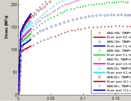
Plot area - data plots and their corresponding models.


To fit the damage model to experimental data, the general strategy is to work the GUI regions in the following order: Datasets; Loading parameters; Solution settings; Yield and yield adjustment constants; Kinematic hardening and recovery constants; Isotropic hardening and recovery constants; Cyclic hardening and recovery constants; Torsional, Compression and Tension constants; then Damage constants including grain size and porosity-damage exponents. The following sequence of steps is typical:

1. Load all experimental datasets. For each dataset, establish the experiment settings (initial temperature, strain rate, stress units, etc), loading parameters, and fixed constants.


2. Start by fitting the experimental dataset with the lowest temperature and lowest rate. Temporarily exclude the rest of the datasets. If there are different tests, fit the compression datasets first, followed by tension datasets, then torsion datasets.


3. For the first dataset, adjust the constants as follows: yield C3; kinematic hardening C9 and recovery C7; isotropic hardening C15 and recovery C13.


4. Restore second dataset. If it has a different temperature than the first, adjust the constants as follows: {C3, C4} if yield is temperature dependent; then {C10, C8, C16, C14}. If the dataset has a different strain rate, adjust C1 and C5 if yield is strain rate dependent, then {C9, C7, C11} and {C15, C13, C17}.


5. Repeat step 4 for the rest of the datasets. If adjusting the temperature dependence constants (even Cs) does not produce good models for high temperature data, adjust C19 and C20. Adjust torsion, compression and tension differentiation constants, if adding stress state dependent experimental data.


6. Adjust damage constants. To track the evolution of the damage state variable, specify the index of the state variable in iretsv under Solution settings. Readjust constants in other boxes as necessary.


7. Record your results. Select Output | Restart file to create a record of your session, to resume it later. Select Output | Constants to ABAQUS input deck merge the material constants into an ABAQUS input deck. Select Output | Parameters and constrains to create a text file record of the fitted constants, which may be used as starting values in future fitting sessions.

Menu items

Help

• Topics - Display the help file on a browser.


• License - Display the license file on a browser.


• About - Display the current version of the tool and the contact information of the developer/maintainer.


• Reset – Re-initialize the tool in case something goes wrong. Data and properties loaded, as well as revised settings, will be lost if not written to files (see Output).

Input

• Restart file (*DMG_restart.mat) - Open a file selection dialog for the name of a “restart” file to be retrieved into the application. A restart file is a record of the state of a previous model fitting session. This file is created by the menu item Output | Restart file during that session. Loading the restart file effectively resumes the previous session.


• Dataset file (*DMG.data) - Open a file selection dialog for the name of a DMGfit dataset to be retrieved into the application. This is a text file containing measurements from a stress-strain experiment, loading information, material constants, and microstructure information. See the Appendix for an example.


• Parameters and constraints file (*DMG.props) - Open a file selection dialog for the name of a “parameters and constraints” file to be retrieved into the application. This is a text file containing lines with the format "name=value fix min max", where name is a fitted constant in the model, fix is 0 or 1 to indicate that the value is to be fixed during optimization, and [min, max] is the range of permissible values for the constant if fix=0. This file may be created through the menu item Output | Parameters set from the parameters displayed in the GUI. See the Appendix for an example.


• Constants & stress-strain from ABAQUS - Retrieve stress-strain generated by a one-element ABAQUS simulation, and use the appropriate entries in the 'USER MATERIAL, CONSTANTS' section of the input deck as the fixed constants for the material.


• Stress-strain from Excel file - Retrieve stress-strain data from a MS Excel file.


• WSMAL legacy data - Retrieve stress-strain data from legacy WSMAL data sets.


• Dataview exported data - Retrieve stress-strain data exported from Dataview.


• A text restart file - Retrieve stress-strain data and fitted parameters from a text restart file created with an earlier version of DMGfit.


• No data; make a curve

• Estimate C3 and C4 - Estimate C3 and C4 from yields of two stress-strain experiments with different temperatures at the same strain rate.


• Use fminsearch – Set options for MATLAB's fminsearch(), then use it as the optimization routine. This routine attempts to find a minimum of a scalar function of several variables, starting at an initial estimate, using a derivative-free simplex search method. This method may find solution outside of the specified parameter ranges.


• Use lsqnonlin – Set options for MATLAB's lsqnonlin(), then use it as the optimization routine. This routine solves nonlinear least-squares curve fitting problems. The default algorithm is a subspace trust-region method and is based on the interior-reflective Newton method.


• Use fmincon – Set options for MATLAB's fmincon(), then use it as the optimization routine. The routine attempts to find a constrained minimum of a scalar function of several variables starting at an initial estimate. The technique is generally referred to as constrained nonlinear optimization or nonlinear programming.


• Use patternsearch – Set options for MATLAB's patternsearch(), then use it as the optimization routine. This routine finds the minimum of a function using pattern search.


• Use genetic algorithm – Set options for MATLAB's ga(), then use it as the optimization routine. This routine finds the minimum of a function using genetic algorithm.


• Check parameter bounds - Before running an optimization, check that the initial parameters are withing their specified [min, max] ranges.


• Enable parallelism – Enable parallel processing in multi-core laptops and desktops. A dialog box will appear to ask you "How many labs?" Here, you specify the number of cores in your machine to be used by DMGfit during optimization. Make sure your machine is well ventilated when using this feature; it may get hot. See Parallelism in DMGfit

• Plot strategy - Specify how many plots to display:


• One dataset per plot - if you're working with a few datasets.


• Same type datasets in one plot - tension datasets in one plot, compression datasets in another plot, etc.


• All datasets in one plot - cluttered if working with several datasets.
• Toggle Hide|Show models - Enable or disable plotting of the model curves.


• Toggle Hide|Show plot legends - Enable or disable plot legends.


• Change font name - Set the font style; fonts in the plot area will be changed when the plot is updated.


• Change font size - Set the font size; fonts in the plot area will be changed when the plot is updated.


• Toggle TeX labels - Toggle between ordinary text or TeX math symbols for the parameter labels.

• Restart file (*DMG_restart.mat) - Open an input dialog for the name of a “restart” file to be created by the tool. This will be a binary file that records the state of the model fitting session (the datasets loaded, the parameter sets attempted, and the solution settings). The extension _DMG_restart.mat is automatically appended to the filename. This file may be loaded at some future time using the menu item Input | Restart file to resumes the session. This feature is useful if the user gets tired and wishes to continue the fitting session after getting some sleep.


• Dataset (*DMG.data) - Open a dialog to select the dataset for which a data file will be created by the tool. This will be a text file containing material identifier, material constants, microstructure information, loading information, and experimental data. Descriptions of the information are included. The extension _DMG.data is automatically appended to the filename. This menu item is useful for creating templates of data files from a restart file.


• Parameters and constraints (*DMG.props) - Open an input dialog for the name of a “properties and constraints” file to be created by the tool from the parameter set currently displayed in the GUI. Descriptions of the properties are included. This will be a text file containing lines with the format "name=value fix min max", where name is a fitted constant in the model, fix is 0 or 1 to indicate that the value is to be fixed during optimization, and [min, max] is the range of permissible values for the constant if fix=0. The extension _DMG.params is automatically appended to the filename. This file may be loaded into the application in the future using the menu item Input | Parameters and constraints. This menu item is useful for creating a template for an input parameter set from a restart file or from the parameter set currently on display in the GUI.


• Constants to ABAQUS input deck (*.inp) - Merge the model parameters into an existing ABAQUS input deck.


• PamStamp2G Material Card - Create stress-strain curves using the PamStamp2G Material Card format.


• Postprocessing information - Open an input dialog for the name of a “postprocessing information” file to be created by the application. This will be a text file of comma separated values, and is suitable for import into a spreadsheet program like MS Excel. The file will contain the model parameters currently on display, the datasets used in fitting the parameters, and the model points. Such post-processing information is typically used to produce publication-quality plots of the model points, or for "cut-and-paste" into a report. The DMG.txt extension is automatically appended to the filename.


• Snapshot to printer - Open a “print preview” of the application window. A snapshot of the window can then be sent directly to a printer.

Quit

• Right away – Turn off parallel processing if previously enabled, then exit the application.


• After writing a restart file – Output a restart file (automatically named “LAST_SESSION-DMG_restart.mat”), turn off parallel processing if previously enabled, then exit the application.


• Reset only (same asHelp | Reset) – Re-initialize the application in case something goes wrong. Data and properties previously loaded into the application, as well as revised settings, will be lost.

Dataset controls

A DMGfit data set is a file that contains experimental stress-strain data, descriptive elements of the experimental sample, the loading parameters to simulate the stress-strain data, and the fixed constants associated with the sample. A data set file is retrieved from disk using Input | Dataset file (*DMG.data). The information contained in the file are automatically displayed when the data set is selected using the DATA SET popup.

The stress-strain data is described by the following elements. Hovering the mouse pointer over an edit box causes a pop-up describing the element to appear. Except for the stress-strain data which are plotted, the elements may be edited directly. Changes will take effect after clicking Apply changes.

• Material - a descriptive name for the material.


• Source - who provided the experimental data.


• Comment - any remarks about the data or the experiment.


• Sample - a tag to differentiate data sets.


• Test type - 1=Tension, 2=Compression, 3=Torsion, 4=Tension+Compression, 5=Compression+Tension


• Units - stress units: 1=psi 2=Ksi 3=Pa 4=KPa 5=MPa 6=GPa


• Tinit - initial temperature.


• Rate - strain rate.

Some constants in the damage model are fixed for the material. These are obtained from the literature or measure from the sample used in the experiment. The fixed constants associated with a sample are automatically displayed upon selection of the data set. These values may be edited directly. Changes will take effect after clicking Apply changes. Hovering the mouse pointer over a value causes a pop-up describing the constant to appear.

• G - Shear modulus (default: 0)


• Bulk - Bulk modulus (default: 0)


• a - Constant to adjust shear modulus due to variation of temperature from initial (default: 0)


• b - Constant to adjust bulk modulus due to variation of temperature from initial (default: 0)


• Tmelt - Melt temperature (K) (default: 3000)


• heat - Heat generation term (default: 0.34)


• Kic - Particle fracture toughness (default: 1000)


• nv - Particle McClintock damage constant (default: 0.3)


• dn - Particle average size (default: 0)


• fn - Particles volume fraction (default: 1e-3)


• dcs0 - Reference grain size or dendrite cell size (default: 30)


• dcs - Grain size or dendrite cell size of experiment sample (default: 30)


• r0 - Initial radius of a spherical void (default: 0)


• volF - Initial void volume fraction (default: 0)

Tips:

1. If G or Bulk is 0, a model will not be generated for the data set.


2. The constant fn and dcs0 should not be 0 because these are used as divisors in the UMAT.


3. If r0 and volF are 0, the damage constants will have no effect on the model.


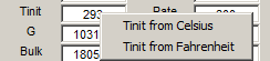
4. A right-click on Tinit exposes a context menu to calculate the value from Celsius or Fahrenheit.



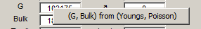
5. A right-click on G or Bulk exposes a context menu to calculate the bulk and shear moduli from the Youngs modulus and Poisson ratio if these are the known quantities.



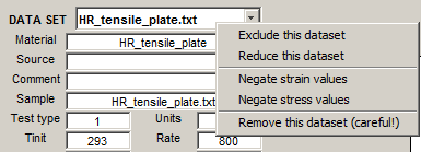
6. A right-click on the DATA SET popup exposes a context menu for some operations on the dataset on focus.



• Exclude this dataset - inhibits the data set on focus from being plotted and fitted. The data set tag is annotated with "(excl)". If an excluded data set is selected for focus, this menu item changes to Restore this dataset, for the opposite effect.


• Reduce this dataset - (see Reducing a dataset).


• Negate strain values and Negate stress values - if the data set on focus has Test type=2 (compression) and the stress-strain data are negative, it is necessary to "flip" the data so that the strain and stress values become positive.


• Remove this dataset (careful) - deletes the data set on focus from memory.

Stress-strain data

An example DMGfit dataset is File:Comp297 DMG.data.

For compatibility with the original BFIT, text files with the following formats for stress-strain data are recognized:

• Two-column
  <strain> <stress>
  <strain> <stress>
  ...


• Four-column
  <stress> <strain> <rate> <temp>
  <stress> <strain> <rate> <temp>
  ...

The other elements of the data set (Material, Source, Comment, Initial temperature, Strain rate, etc) may be entered using the Data set controls.

DMGfit is able to load stress-strain data from Excel files. Use the menu item Input | Stress-strain from Excel file to open an MS Excel file and read a rectangular array of numbers. Column indices for the strain and stress values and other data set elements are specified in the subsequent dialog.

Use the menu item Output | Dataset to create a template for data files from a loaded data set. Data files so created may later be loaded using Input | Dataset file.

Reducing a dataset

A data set with thousands of data points will require long running time for the fitting procedure since an estimate of the error at each point has to be calculated. The running time may be decreased by reducing the number of stress-strain pairs in the data set.

The DATA SET context menu Reduce this dataset disables all controls and makes visible the controls to perform the reduction operation.


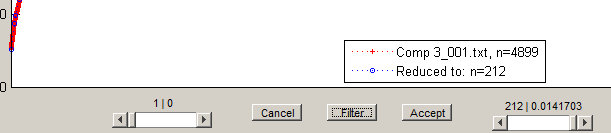
The left slider moves the left endpoint, while the right slider moves the right endpoint.

The Filter button invokes a filtering routine to find points such that a line drawn between the points approximates the data between those points to a relative error not exceeding the filter tolerance. For comparison, the points found are superimposed on the original dataset.

Cancel discards changes to the data set, deactivates the reduction controls, and enables the rest of the controls.

Accept creates a new data set from the filtered/reduced stress-strain data points of the data set on focus, prefixing "reduced-" to the tag. The data set on focus is automatically excluded, and the reduced data set becomes the focus.

Loading Parameters

A set of loading parameters is associated with each experimental data. These parameters are used by the UMAT Driver to model the experiment.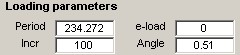


The values of the parameters are automatically displayed upon selection of a data set. Hovering the mouse pointer over a label causes a pop-up describing the parameter to appear. The loading parameter values may be edited directly. Changes will take effect after clicking Apply changes.

Descriptions of the loading parameters:

• Period - simulation time period; the final simulated strain value will be (Period*Rate)


• e-load - for Test type=4 or 5; the strain value where the load direction changes; otherwise 0.


• Incr - number of strain increments for the simulation; the execution time of the simulation is directly proportional to this value.


• Angle - the bi-axial loading ratio.

Tips:

1. If Period is 0, a model will not be generated for the data set.


2. If a model curve is a "zigzag" or is "wavy", increase the Incr parameter for the corresponding dataset.


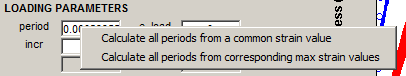
3. A right-click on Period exposes the context menu to automatically calculate all periods so that all data models will end at a common strain value, or at the respective final strain values.

For example, in the figure below, the periods were automatically computed to model up to strain=0.02.

Solution Settings

In addition to the loading parameters, the UMAT Driver requires the solution settings to model an experimant. Notable among these is iretsv, the index to the state variable to be plotted along with the model stress-strain curve.

Parameter Study Controls

A right-click on the current value of a fitted parameter activates the parameter study controls and disables the rest of the DMGfit controls.

For example, a right-click on activates the parameter study controls with the following initial values.


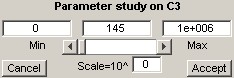
The range constraint for C3 is transferred to the Min and Max edit fields as well as to the slider limits. The current value is transferred to the Current edit field and is used to initially position the slider.

The Min, Current and Max values may be edited directly. Changes will take effect after clicking anywhere in the window outside of the edit boxes.

Operating the slider decreases or increases the Current value, depending on where the slider bar is positioned. The model plots are updated automatically with each change of the current value.

If the Min value is close to the Max value, the slider may not work properly due to the resulting low resolution of the slider steps. In this case, setting the Scale (value beside *10^) to a negative integer may restore the expected functionality. Similarly, for a large range of values, setting the scale to a positive integer may prevent huge jumps in Current when the slider is operated.

Accept creates a new parameter set from the set currently on focus, where the current value and range constraint for the selected model parameter are transferred from the parameter study controls. This also exits the parameter study.

Cancel exits the parameter study without any change to the selected model parameter.

Parameter Set Controls

DMGfit keeps track of the sets of fitted parameters attempted during a session.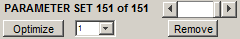


The PARAMETER SET slider selects which parameter set which will be on focus. This is the set used to generate the model plots on display.

Remove discards the parameter set currently on focus from memory, renumbering the succeeding sets, if any. The next available parameter set becomes the focus.

Optimize invokes the optimization routine to automatically update the values in the parameter set. See Parallelism in DMGfit for an explanation of the function of the pop-up beside Optimize.

Apply changes commits changes to any displayed value (experiment descriptions, loading parameters, fixed constants, fitted constants) or check box in the GUI. If one or more fitted parameters are manually changed, a new parameter set is created from the displayed values. The new set automatically becomes the parameter set on focus.

Fitted Parameters

For each fitted constant, there are three controls: the label static text, the current value edit box, and the fix check box.

For example, consider .Hovering the mouse pointer on the edit box will activate a popup that displays a description and current range constraint for the constant.


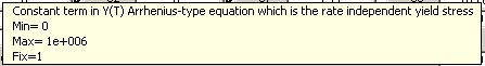
The current value can be changed directly. The change will not take effect until Apply changes is clicked.

A right-click on the current value activates the single Parameter study controls and disables the rest of the DMGfit controls.

If the check box is unchecked, the parameter may be updated when is clicked. If checked, the parameter will be fixed (not changed) by the optimization routine.

Descriptions of the fitted parameters:

• C1 - Constant term in V(T) Arrhenius-type equation which determines the magnitude of rate dependence on yielding (units=MPa)


• C2 - Temperature dependent activation term in V(T) Arrhenius-type equation (units=Kelvin)


• C3 - Constant term in Y(T) Arrhenius-type equation which is the rate independent yield stress (units=MPa)


• C4 - Temperature dependent activation term in Y(T) Arrhenius-type equation (units=Kelvin)


• C5 - Constant term in f(T) Arrhenius-type equation which determines the transition strain rate from rate independent to dependent yield (units=1/sec)


• C6 - Temperature dependent activation term in f(T) Arrhenius-type equation (units=Kelvin)


• C7 - Constant term in rd1 equation which describes the kinematic dynamic recovery (units=1/MPa)


• C8 - Temperature dependent activation term in rd1 equation (units=Kelvin)


• C9 - Constant term in h1 equation which describes the kinematic anisotropic hardening modulus (units=MPa)


• C10 - v term in h1 equation (units=MPa/Kelvin)


• C11 - Constant term in rs1 equation which describes the kinematic static recovery (units=1/(MPa sec))


• C12 - Temperature dependent activation term in rs1 equation (units=Kelvin)


• C13 - Constant term in rd2 equation which describes the isotropic dynamic recovery (units=1/MPa)


• C14 - Temperature dependent activation term in rd2 equation (units=Kelvin)


• C15 - Constant term in h2 equation which describes the isotropic hardening modulus (units=MPa)


• C16 - Temperature dependent activation term in h2 equation (units=MPa/Kelvin)


• C17 - Constant term in rs2 equation which describes the isotropic static recovery (units=MPa/sec)


• C18 - Temperature dependent activation term in rs2 equation (units=Kelvin)


• C19 - Multiplication term in equation 1 + tanh(c19(c20-T)), which is an adjustment to the yield strength over a large temperature range (units=1/Kelvin)


• C20 - Used in yield strength adjustment equation (units=Kelvin)


• C21 - Long range kinematic dynamic recovery rd3 (units=1/MPa)


• C22 - Temperature dependent activation in rd3 dynamic recovery equation (units=Kelvin)


• C23 - Long range kinematic hardening h3 (units=MPa)


• C24 - Temperature dependent activation in h3 equation (units=MPa/Kelvin)


• C25 - Long range kinematic static recovery rs3 (units=1/(MPa sec))


• C26 - Temperature dependent activation in rs3 static recovery equation (units=Kelvin)


• Ca - Torsional softening constant in kinematic and isotropic hardening and dynamic recovery equations


• Cb - Tension/compression asymmetry constant in kinematic and isotropic hardening and dynamic recovery equations


• an - Torsional constant a in void-crack nucleation model


• bn - Tension/compression constant b in void-crack nucleation model


• cn - Triaxiality constant c in void-crack nucleation model


• Z - Grain size or dendrite cell size exponent


• Ccoef - Coefficient constant in void-crack nucleation model


• cd1 - Void impingement coalescence factor, D=nucleation*void volume*coal


• cd2 - Void sheet coalescence factor, D=nucleation*void volume*coal


• NTD - Void-crack nucleation Temperature Dependence


• CTD - Void coalescence Temperature Dependence


• CAcon - Cocks Ashby void growth constant


• beta - Porosity damage exponent

Tips:

1. Leave C5 to the default nonzero value if yield is NOT strain rate dependent. C5=0 does not produce a good model.


2. Several values can be modified and/or fixed at the same time. The changes will take effect after Apply changes is clicked. A new parameter set is created from the set on focus, using the updated values. The new set automatically becomes the focus.


3. Depending on the optimization routine, a parameter that has a value of zero may be respected, and may remain zero even if it is not fixed. For the constant to participate in fitting, set it initially to a "small" non-zero value.


4. The group ordering of the constants in the GUI suggests a strategy for fitting. After establishing the fixed model constants, the suggested order for the parameters to be fitted is:


1. Yield and yield adjustment parameters,


2. Kinematic hardening and recovery parameters,


3. Isotropic hardening and recovery parameters,


4. Long range hardening and recovery parameters,


5. Torsional, Compression & Tension differentiation parameters, and


6. Damage parameters.

Plot Area

Data plots for "active" datasets will appear in the Plot Area. The plots of the corresponding models will also appear if the Toggle Hide|Show models switch is enabled. Plot legends will also appear if the Toggle Hide|Show plot legends switch is enabled. See Plot strategy in Display for other options.

A right-click on a blank spot in a plot activates a context menu for additional plot options.


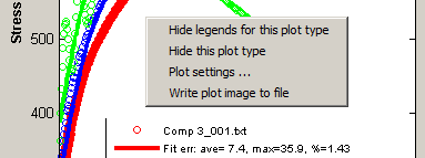
Hide legends for this plot - hides the legends if these get in the way. Next time the context menu is activated, the menu item changes to Show legends for this plot. For finer control on the location of the legends, see Plot settings... below.

Hide this plot type - excludes all datasets of the selected dataset type; thus, the data and model plots for these datasets will not appear. To restore, select an excluded dataset using the DATA SET popup, then right-click the popup to expose the context menu, then select Restore this dataset. See Dataset controls.

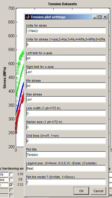
Plot settings... - activates a dialog to set options for the plot.


Write plot image to file - creates a TIF image file from the DMGfit window. Use #Output | Snaphot to printer for finer control over the appearance of the image, and to be able to send the image file to a printer.

Parallelism in DMGfit

When parallel-enabled (see Optimization | Enable parallelism), the manner in which DMGfit utilizes multiple cores depends on the setting of the pop-up menu beside the Optimize button(). This pop-up determines the number of starting solutions when you click Optimize.

IF you specify one starting solution (i.e., "Optimize 1") AND you specify "Use fmincon" or "Use patternsearch" or "Use genetic algorithm" as the optimization method, THEN DMGfit will use the multiple cores. The starting solution for the optimization are the displayed parameters, and the final solution is whatever the optimization method will find when starting from these parameters. The methods fmincon, patternsearch and genetic algorithm have parallel implementations in MATLAB; hence, the optimization process will benefit from the multiple cores. The methods fminsearch and lsqnonlin DO NOT have parallel implementations (as of MATLAB R2012a), so optimization with these methods will NOT benefit from multiple cores with "Optimize 1" (however, these will still find final solutions).

IF you specify "Optimize N", then DMGfit will automatically generate a number of starting solutions as follows. Let K be the number of DMGfit parameters that are NOT fixed (i.e. unchecked in the DMGfit user interface). The "global" search space for the optimization is the K-dimensional hyper-rectangular region

R = [min_1,max_1] * [min_2,max_2] * ... * [min_K,max_K],where [min_i,max_i] is the range for the i-th parameter. DMGfit will divide each range will into N subintervals so that there will be N^K (N to the power K) hyper-rectangular subregions.

DMGfit will generate a random starting solution within each subregion, and run an optimization from the random starting point. The optimization will be bounded by the limits of the subregion (except if the method is fminsearch).

The following is a small table for N^K, the number of optimization runs to be performed by DMGfit. Since one run might take several seconds or a few minutes, the whole process may still require a significant wait even if DMGfit will perform the runs in parallel.

DMGfit will collect a number of "locally good" results, along with the limits of the subregions returning such results. When all the N^K searches are complete, you can browse the results and manually decide which are "really good". Not all subregions will produce "good" results; hence, much much less than N^K results will be returned.

N^K	K=2	K=3	K=4	K=5	K=6	K=8	K=10	K=12
N=2	4	8	16	32	64	256	1024	4096
N=3	9	27	81	243	729	6561
N=4	16	64	256	1024	4096
N=5	25	125	625	3125

Thus, "Optimize N" is intended to be used with "small N" and "small K" for semi-automated exploration of the search space, if you have no idea what are "reasonable combinations of limits" for the model parameters.

References

• Bammann, D. J., "Modeling Temperature and Strain Rate Dependent Large of Metals," Applied Mechanics Reviews, Vol. 43, No. 5, Part 2, May, 1990.


• Bammann, D. J., Chiesa, M. L., Horstemeyer, M. F., Weingarten, L. I., "Failure in Ductile Materials Using Finite Element Methods," Structural Crashworthiness and Failure, eds. T. Wierzbicki and N. Jones, Elsevier Applied Science, The Universities Press (Belfast) Ltd, 1993.


• Cariño, R., Horstemeyer, M., & Burton, C. (Dec 2007). Re-engineering DMGFIT – Fitting Material Constants to Internal State Variable Models. MSU.CAVS.CMD.2007-R0040.


• Horstemeyer, M., Carino, R.L., Hammi, Y., & Solanki, K.N. (Jun 2009). MSU Internal State Variable Plasticity-Damage Model 1.0 Calibration, DMGfit Production Version Users Manual. MSU.CAVS.CMD.2009-R0010, Mississipi State University: CAVS.


• Horstemeyer, M.F., Lathrop, J., Gokhale, A.M., and Dighe, M., “Modeling Stress State Dependent Damage Evolution in a Cast Al-Si-Mg Aluminum Alloy,” Theoretical and Applied Fracture Mechanics, Vol. 33, pp. 31-47, 2000.


• Lathrop, J.F., (Dec 1996). BFIT—A Program to Analyze and Fit the BCJ Model Parameters to Experimental Data Tutorial and User’s Guide. SANDIA REPORT SAND97-8218 . UC-405, Unlimited Release, Printed December 1996.


• MATLAB - link