
Integrated Computational Materials Engineering (ICME)
Intermediate Strain-Rate Testing of ASTM A992 and A572 Grade 50 Steel
Abstract
Uniaxial tension tests were conducted on ASTM A572-50 and A992 steel at
increasing strain rates to determine material strength properties of structural
members subjected to dynamic loadings. The increase in dynamic yield strength
and ultimate tensile strength, defined as the dynamic increase factor (DIF),
versus strain rate was determined to provide the necessary information to
efficiently design blast resistant structures utilizing modern day structural
steel. Dynamic strength properties were determined by high-rate tensile tests
using a hydraulic testing apparatus and compared to static values obtained from
ASTM E8 standard tension tests. The comparisons were used to calculate the DIF
of each steel at strain rates ranging from 0.002 to 2.0 inch/inch/second.
Experiments revealed that A572-50 steel exhibited an increase in yield strength
up to 35% and ultimate tensile strength up to 20% as strain rate increased over
the range tested. A992 steel exhibited a similar increase in yield strength up
to 45% and ultimate tensile strength up to 20%. DIF versus strain rate curves
obtained during this research will be used to develop criteria within the
structural steel design chapter of Unified Facilities Criteria (UFC) 3-340-02
(2014) for A572-50 and A992 steel.
Truncated presentation of "Effects of High Strain Rates on ASTM A992 and A572
Grade 50 Steel" [1].
"High" strain rate classification applies to shock-induced blast loading
community. Actual strain classification is ~intermediate strain rate.
Test Methods
Test Specimen
ASTM A572-50 specimens were fabricated from a domestic, nominal 0.375-in.-thick plate. The mill test report (MTR) indicated that the plate also met the specifications of ASTM A709-50. ASTM A992 specimens were obtained from the web of domestic S12x31.8 beams, which had a nominal thickness of 0.35 in. The MTR for the A992 steel indicated the beam also met specifications of ASTM A6, A709-50, A572-50, and A36. The chemical composition (weight percent) of the tested materials is listed in the table below, as specified by the MTRs.
| Material | C | Mn | P | S | Si | Al | Cu | Ni | Cr | Mo | Cb/Nb | V | Ti |
|---|---|---|---|---|---|---|---|---|---|---|---|---|---|
| A572-50 Plate | 0.17 | 1.04 | 0.009 | 0.002 | 0.19 | 0.027 | 0.22 | 0.19 | 0.12 | 0.07 | 0.001 | 0.042 | 0.002 |
| A992 Beam | 0.07 | 1.21 | 0.01 | 0.022 | 0.2 | 0.001 | 0.28 | 0.1 | 0.1 | 0.048 | 0.001 | 0.031 | - |
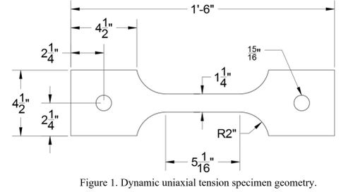
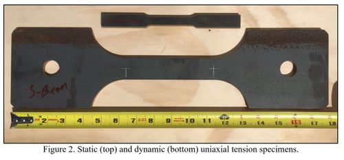
Static-rate specimen were waterjet cut to ASTM E8 standard sheet-type geometries. Dynamic-rate specimens were waterjet cut into a modified pin-type specimen geometry shown in Figure 1 with tolerances similar to those in ASTM E8. The full thickness of the parent material was used. Bolt holes were drilled using a computer numerical control (CNC) machine. Figure 2 provides a visual comparison of the static and dynamic specimens.
Equipment
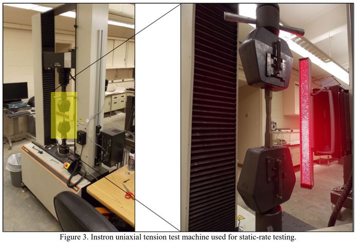
The U.S. Army Engineer Research and Development Center's (ERDC) Instron 33R4206 Universal Testing System (Figure 3) was used to conduct the static, uniaxial tension tests. An integrated optical extensometer was used to record elongation over time. The apparatus allowed controlled-rate testing at an average elastic strain rate of approximately 0.00002 s-1.
Dynamic Tension Test Apparatus
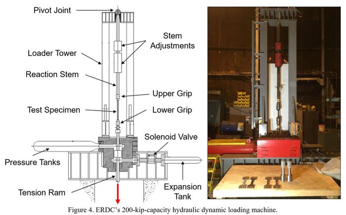
ERDC’s 200-kip-capacity hydraulic loader (Figure 4) was used to conduct the
dynamic, uniaxial tension tests. This loader has been employed by ERDC to
conduct dynamic experimentation on reinforcing steel, splices, and fasteners
since the 1970’s, and it remains the approved validation apparatus for the
dynamic testing of mechanical splices for reinforcing steel used in protective
design.
The device was slowly pressurized by pumping compressible silicon oil into the
top and bottom pressure chambers. Pressure in the top chamber was kept at a
slightly higher pressure in order to maintain a small tensile preload (50-1,000
lbf) on the specimen. The measured preload ensured alignment of the specimen
through the bolted connections and also seated the top reaction stem pivot
joint to further ensure axial loading of the specimen. Once the desired fluid
pressure was reached, a quick-opening valve leading to an empty expansion tank
was opened. Pressure in the lower chamber was rapidly reduced allowing the
piston to translate downward and apply a tension load to the specimen attached
above. Flow rate of the fluid in the lower chamber into the expansion tank was
controlled by an adjustable orifice and was the main variable in changing the
loading rate (strain rate) applied to the test specimen.
The adjustable orifice allows for specimen strain rates of approximately 0.001
to 4.0 s-1, and the limits are dependent on specimen geometry,
specimen stiffness, and oil pressure. The lowest strain rate recorded during
experimentation was 0.002 s-1 with the smallest obtainable orifice
setting, and the highest was 2.91 s-1 with the largest orifice setting. The UFC
lists strain rates for bending, tension, and compression modes at various
pressure levels. Provided strain rates range from 0.02 to 0.30 s-1,
and were well within the strain rate limits of the hydraulic loader.
Instrumentation
StrainAxial deformation was measured using a Phantom Miro 320S high-speed (HS)
camera. The HS camera recorded locations of gauge marks from time zero
(trigger) through fracture of the specimen. The video was uploaded into Image
System’s TrackEye Motion Analysis (TEMA) software, which incorporated an
optical extensometer feature that tracked each gauge mark location, represented
by a single pixel, frame by frame throughout the length of the video recording.
The software then output the distance between gauge marks (elongation) with
respect to time as they moved from pixel to pixel. Quadrant markers were added
to the specimen to enhance the tracking capabilities of the TEMA software.
Pixel length was determined by the vertical resolution of the HS camera
recording and the distance between the tracked points. The vertical resolution
was set to the maximum of 1,200 pixels, which provided an elongation
measurement accurate to approximately 0.00105 in., or 185 microns of strain,
for the rates of 0.002 to 0.05 s-1. At higher strain rates, the
collection rate was increased, forcing the vertical resolution to be reduced to
904 pixels, which allowed an approximate accuracy of 0.00155 in. for elongation
and 255 microns for strain. The HS camera software was calibrated to remove
error due to lens distortion using the prescribed TEMA lens calibration
guidelines.
Even with a collection rate of 13,000 frames per second, for experiments
conducted at the highest rate (≈ 2.0 s-1) the HS camera was
only able to obtain roughly 20 data points before the specimens would yield.
Bonded strain gauges were implemented at this rate to obtain high resolution
strain data up to yield to supplement the HS Camera data. Strain gauges were
applied to specimens used for strain rate calibration and specimens tested at
2.0 s-1. For these specimens, it was necessary to remove mill scale
from the parent material to facilitate strain gauge bonding. Approximately
0.006 in. (< 2% of thickness) of material was removed by machining across
the entire gauge region, which allowed application of a strain gauge to the
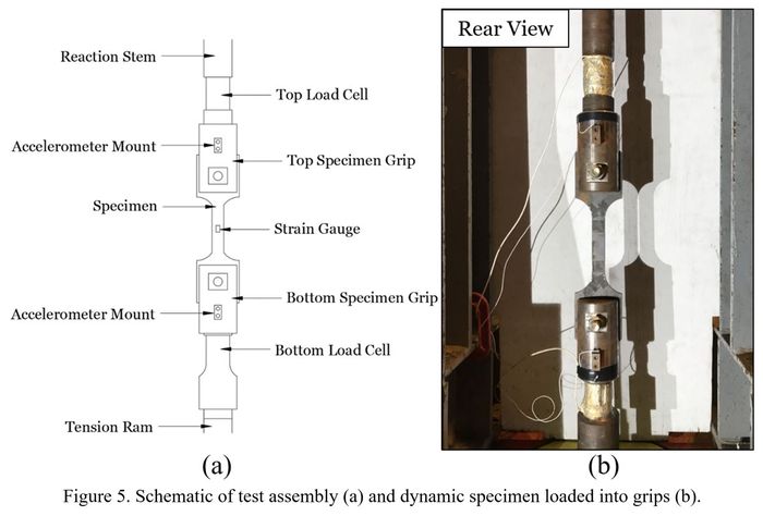
exposed steel at the center of the gauge region. A schematic of the test
assembly showing the dynamic specimen and locations of instrumentation is shown
in Figure 5.
Load was measured using two load cells in series with the 200-kip-loader tension ram. The load cells were fabricated from AISI 4130 quenched and tempered steel with a minimum yield strength of 100 ksi. The bridge network used on the load cells consisted of eight strain gauges installed in pairs at the quarter points, midway in the necked down portion of the load cell. One gauge of each pair measured axial strain and the other measured Poisson’s effect. The active gauges were on the opposite sides of the bridge topology with the adjacent Poisson gauges electrically connected on opposite sides as well. Calibration of the load cells was conducted by placing both in series with a pre-calibrated, manufactured load cell. The load cells were statically calibrated to a maximum load of 200 kip. Post-test verification indicated that the load cells maintained calibration throughout all dynamic experiments.
AccelerationTwo accelerometers (Meggit, model 7280A) were used to record acceleration during experiments conducted at rates of 0.05 s-1 and higher. Data recorded from these devices allowed inertial load effects to be determined and removed from the load versus time history. Accelerometers were mounted in an orientation that measured positive acceleration in the upward direction.
Load Analysis and Data Reduction
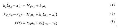
Inertial Force CorrectionNewton’s second law explains that when force is applied to objects with mass, inertial forces develop to resist the impending motion. If the objects have a large mass or if the accelerations are high, these inertial forces become quite significant. When the tension ram of the testing machine began to first apply rapid load onto the specimen through the lower grip, the mass of the grip and specimen resisted the downward acceleration. Increased load was required to overcome this inertial resistance and begin pulling the lower grip and half of the specimen downward applying tension. The lower load cell recorded, as one total load, both the applied load to the specimen and the load required to overcome inertia. Inertial force was subtracted from the bottom load cell record to form a corrected load applied to the specimen. Contrarily, addition of inertial force was required for the top load cell record to form the corrected load applied to the specimen. An uncoupled (mass) spring-mass model (Figure 6) was used to develop the required load correction equations. Equilibrium equations (Eq. 1-3) were developed to solve for the corrected load applied to the specimen.
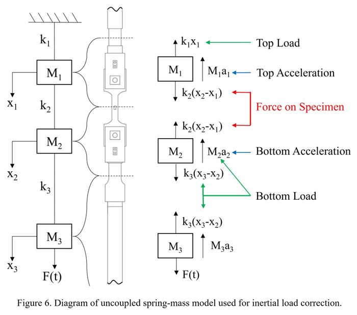
where:
F(t) = applied force as function of time (lbf)
M1 = mass of top specimen grip and half of the test
specimen (lbm)
M2 = mass of bottom specimen grip and half of test specimen
(lbm)
M3 = mass of tension ram and piston (lbm)
a1 = acceleration of M1 (g)
a2 = acceleration of M2 (g)
a3 = acceleration of M3 (g)
k1 = spring constant of upper reaction member (lbf/in.)
k2 = spring constant of test specimen (lbf/in.)
k3 = spring constant of tension ram and piston
(lbf/in.)
x1 = displacement of M1 (in.)
x2 = displacement of M2 (in.)
x3 = displacement of M3 (in.)
Eq. 1 represents the corrected load on the specimen using the top load cell and
acceleration data. Eq. 2 was solved to determine the corrected load using the
bottom load cell and acceleration data (Eq. 4).

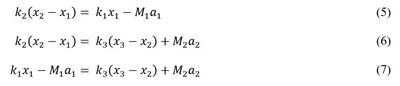
Since the accelerometers were mounted in an orientation that recorded positive acceleration in the upward direction, accelerations in Eq. 1 and Eq. 4 were corrected by switching the signs of a1 and a2 to form Eq. 5 and Eq. 6, respectively. Substitution allows for Eq. 7 to be derived, which states that the corrected load using the top data records, load and acceleration, should theoretically be equal to the corrected load using the bottom data records. Testing at the static rate (0.00002 s-1) and the dynamic rate of 0.002 s-1 produced accelerations of insignificant magnitudes and were therefore neglected.
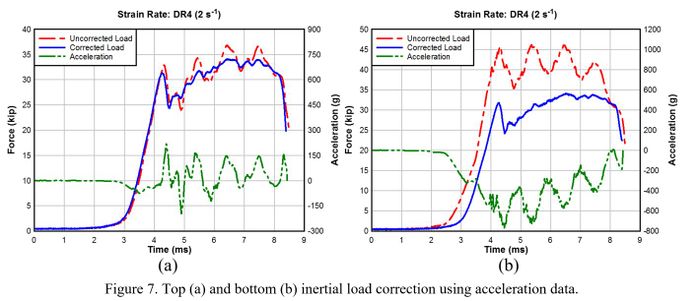
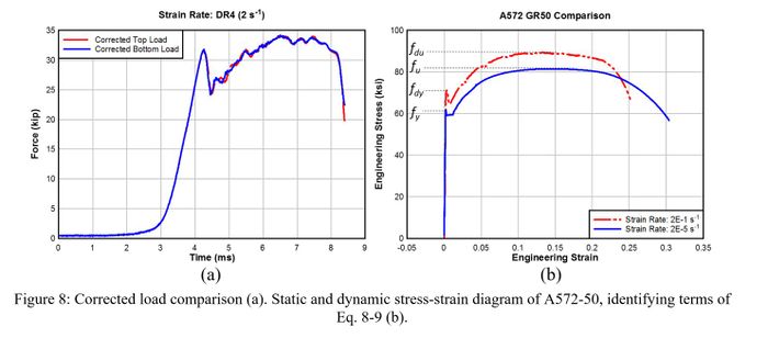
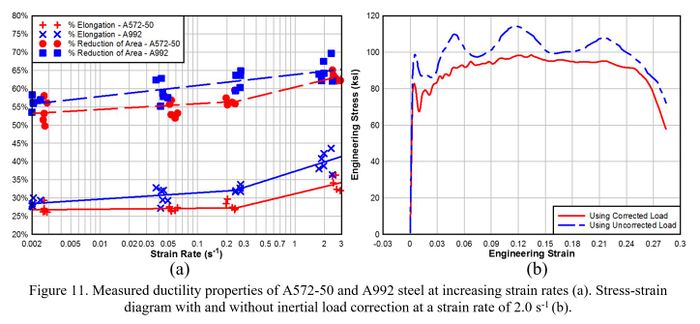
Figures 7-8a shows an example inertial force correction for both the top and bottom load cell data for the highest strain rate experiments (≈ 2.0 s-1). The bottom load cell, attached to the tension ram of the loader, experiences up to four times the acceleration of the upper; therefore, the inertial load correction is much more significant on the bottom load cell data. The average of the corrected top and corrected bottom load versus time histories are used for the calculation of engineering stress.
Data Analysis
The average corrected load was divided by the original cross section of the
test specimen to calculate engineering stress. Average strain was determined
from elongation data. Stress was plotted as a function of strain to develop the
stress-strain diagram for each test. Upper yield strength was determined as the
stress corresponding to the maximum force at the onset of discontinuous
yielding as prescribed in ASTM E8-7.7.3. Ultimate tensile strength was
calculated by dividing the maximum force applied to the specimen during the
test by the original cross-sectional area of the specimen (E8-7.10). The
strength properties were rounded to the nearest 0.1 ksi. Strain rate was
determined by calculating the slope of the strain-time data in the elastic
deformation region.
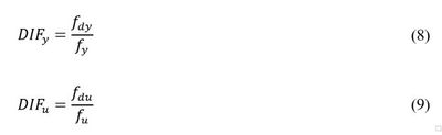
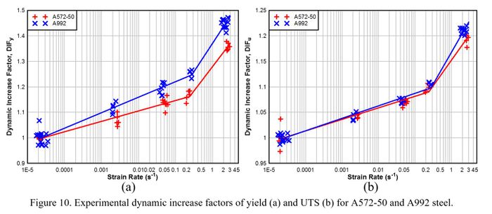
The ratio of dynamic-to-static yield stress is defined as the dynamic increase
factor (DIFy) at a specified strain rate. The tested A572-50 and A992 steels
both exhibited discontinuous yielding. ASTM specifies minimum yield stress
values for these steels based on the yield point; therefore, the yield point
(upper yield strength) was used in determining DIFy using Eq. 8. Figure 8b
indicates the values used in the equations below on a static and dynamic
stress-strain diagram.
where:
DIFy = dynamic increase factor for yield strength for a
particular strain-rate
DIFu = dynamic increase factor for ultimate tensile
strength for a particular strain rate
ƒdy = dynamic yield strength at a particular strain
rate above static (ksi)
ƒdu = dynamic ultimate tensile strength at a
particular strain rate above static (ksi)
ƒy = average yield strength measured during static
testing (ksi)
ƒu = average ultimate tensile strength measured during
static testing (ksi)
Results
Eight static-rate tension tests were originally conducted for each steel.
Six more were required to verify the static properties of a surplus A992 beam
that was obtained to fabricate additional specimens required to complete the
dynamic experiments. A minimum of five dynamic-rate tension tests were
conducted at each rate. In some cases additional dynamic tests were conducted
to compensate for specimens that fractured on gauge marks. A comparison of load
histories between specimens that fractured on gauge marks and those that did
not indicated no identifiable impact on yield strength or UTS; therefore,
results from these experiments were included in the analysis of DIF data.
Ductility properties for the specimen that fractured on gauge marks were
uncharacteristically low and were not included in percent elongation or
reduction of area analysis.
Table 2 lists the number of tension tests conducted at each target strain rate.
The average material strength values and standard deviations for each target
strain rate are listed in Tables 3-4. The strain rate corresponding to each
targeted rate could not be kept constant between tests; however, dynamic yield
and UTS values were obtained without a substantial amount of distribution when
grouped by target strain rate. Standard deviation for the static yield strength
was 0.27 ksi for A572-50 and 1.38 ksi for A992. The static UTS standard
deviation was 1.43 ksi for A572-50 and 0.48 ksi for A992. Deviations for the
dynamic-rate tests were of a similar order of magnitude as the static.
Table 2: Uniaxial Tension Test Matrix
| Material | Target Strain Rate (s-1) | # Tests |
|---|---|---|
| A572-50 | 0.00002 (Static) | 8 |
| 0.002 (DR1) | 5 | |
| 0.05 (DR2) | 8 | |
| 0.2 (DR3) | 5 | |
| 2.0 (DR4) | 6 | |
| Total | 32 |
| Material | Target Strain Rate (s-1) | # Tests |
|---|---|---|
| A992 | 0.00002 (Static) | 14 |
| 0.002 (DR1) | 5 | |
| 0.05 (DR2) | 7 | |
| 0.2 (DR3) | 5 | |
| 2.0 (DR4) | 10 | |
| Total | 41 |
Table 3: Average Material Strength Properties of A572-50 at Increasing Strain Rates
| Target Strain Rate (s-1) | Standard Deviation Strain Rate (s-1) | Average Yield Strength (ksi) | Standard Deviation Yield Strength (ksi) | Average UTS (ksi) | Standard Deviation UTS (ksi) |
|---|---|---|---|---|---|
| 0.00002 (Static) | 2.3E-06 | 61.5 | 0.27 | 81.9 | 1.43 |
| 0.002 (DR1) | 9.4E-05 | 65.7 | 1.37 | 85.4 | 0.36 |
| 0.05 (DR2) | 5.9E-03 | 69.8 | 1.20 | 87.5 | 0.42 |
| 0.2 (DR3) | 2.1E-02 | 71.7 | 1.24 | 89.8 | 0.55 |
| 2.0 (DR4) | 1.8E-01 | 83.5 | 0.85 | 97.9 | 0.90 |
Table 4: Average Material Strength Properties of A992 at Increasing Strain Rates
| Target Strain Rate (s-1) | Standard Deviation Strain Rate (s-1) | Average Yield Strength (ksi) | Standard Deviation Yield Strength (ksi) | Average UTS (ksi) | Standard Deviation UTS (ksi) |
|---|---|---|---|---|---|
| 0.00002 (Static) | 2.3E-06 | 54.0 | 1.38 | 68.9 | 0.48 |
| 0.002 (DR1) | 9.4E-05 | 60.3 | 1.13 | 71.6 | 0.53 |
| 0.05 (DR2) | 5.9E-03 | 64.3 | 1.20 | 73.9 | 0.27 |
| 0.2 (DR3) | 2.1E-02 | 67.6 | 0.70 | 76.2 | 0.18 |
| 2.0 (DR4) | 1.8E-01 | 78.1 | 1.00 | 83.4 | 0.39 |
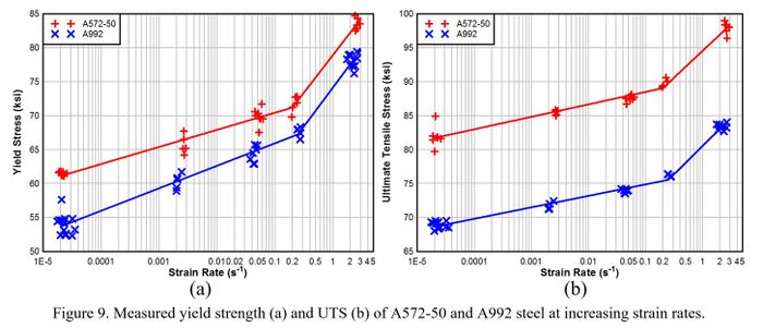
The measured yield strength and UTS for each experiment are shown in Figure 9. Static yield strength (ƒy) and UTS (ƒu) were determined by averaging values obtained from static testing of each material. The DIF for yield (DIFy) and UTS (DIFu) were calculated with Eq. 8 and Eq. 9, respectively. The calculated values were graphed in DPlot software. Analysis of the data led to formulation of a bi-linear least-squares regression curve fit on a log-linear DIF versus strain rate plot. Individual values for each experiment and curve fits are shown in Figure 10. The percent elongation after fracture and percent reduction of area for each experiment are shown in Figure 11a.
Acknowledgments
This research is the product of the U.S. Army Engineer Research and Development Center, Geotechnical and Structures Laboratory and was funded by the Department of Defense Explosives Safety Board.
References
1. Murray, Matthew P, Stephen P Rowell, and Trace A Thornton. 2018 “Effects of High Strain Rates on ASTM A992 and A572 Grade 50 Steel.” In International Explosives Safety Symposium and Exhibition, 2018. San Diego, CA: NDIA. https://ndiastorage.blob.core.usgovcloudapi.net/ndia/2018/intexpsafety/MurrayPaper.pdf.