
×
![Enlarged Image]()
Integrated Computational Materials Engineering (ICME)
Product Design Optimization with Microstructure-property Modeling and Associated Uncertainties
Overview
- What we are trying to achieve? What is an expected outcome?
- How this could advance engineering design?
- What are the challenges?
- in optimizations
- in software engineering
- why do we need a tool?
- What is the expected functionality of the tool?
ATC
Overview of ATC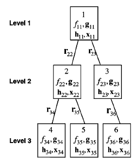
System Structure.
ATC is applicable for problems that have a hierarchical structure so that the top-level design is a supersystem that consists of a number of systems, each of which may consist of its own subsystems. For example, an automobile may be composed of powertrain, body, and chassis, and the power train may be composed of engine and transmission, etc. This model is general enough to account for any number of levels in the hierarchy [10]. The objective function for the overall system can be described as a sum of the objective functions of its components. Typically, the objective function is entirely at the system level. Moreover, the subproblems are nearly separable except for a few linking variables. Figure 1a shows an example. Specifically, a parent and child are connected by a response variable, which represents a child’s response to the design specification that its parent imposes. This “response variable” may or may not be a variable in the original predecomposition formulation: It is typically the output of the subsystem simulator and the input to the system simulator, and it may be treated as an intermediate calculation of the original formulation. The effects of subsystem response on system behavior are what prevent subsystems from being designed independently.
Notation.
Different notations are used in describing and defining ATC, depending on the application [1,10–12]. In this paper, we adopt the notational system of Tosserams et al. [12] for simplicity. Consider a system that can be decomposed into N levels and M elements. The subscript ij is used to denote the jth element of the system in the ith level. fij is the scalar objective function, and gij=<0 and hij=0 are the inequality and equality constraints, respectively. Local variables of element j are denoted by xij. rij is the response of element j calculated by analysis model aij. Generally speaking, this model is an engineering simulation or a set of equations predicting the behavior of the subsystem. Ei is the set of elements at level i, and Cij is the set of children of element j. The system in Fig. 1 is shown corresponding to this notation.
Methods.
- QP: Quadratic Penalty Method
- OL: Ordinary Lagrangian Method
- AL: Augmented Lagrangian Method
- ALAD: Augmented Lagrangian with Alternating Direction Methods of Multipliers
- DQA: Diagonal Quadratic Approximation Method
- TDQA: Truncated Diagonal Quadratic Approximation Method
Benchmark problems
- MLDO with MATLAB
- Problem 1
Outline of the first paper: description of the tool for CS/SE
- MLDO tool design