The Finite Element (FE) setup of the SHPB was akin to the experiment. The striker bar was set in motion to initialize the FE simulation. The speed of the striker bar corresponded to that in the SHPB experiment for a particular strain rate. When the striker bar came in contact with the incident bar, a stress wave was set in motion. Thus, the stress waves that arose from the striker bar’s impact on the incident bar gave different levels of applied pressure. The applied pressure then became the boundary conditions that gave rise to the different strain rates similar to the experiment. The striker, incident and transmitted bars were treated as elastic materials. The Young’s Modulus and Poisson’s ratio were 2391.2 MPa and 0.36 respectively. Figure 1 gives an overview of the FE model that simulated the SHPB test. In Figure 1, the loading direction is along the negative z-axis and the loading direction stress (which is compressive) is denoted by σ₃₃.

Mesh refinement study for the FE model was also conducted to analyze the convergence of ABAQUS/Explicit solutions (Simulia Inc., 2009)[1]. Figures 2 and 3 show plots of incident and transmitted strain measurements respectively, at different mesh resolutions. Figures 2 and 3 illustrate that for a mesh of above 12,432 elements, FE solutions are invariably independent of further mesh refinement. Therefore, the number of elements included were 47300, and the type of elements used were regular hexahedral.

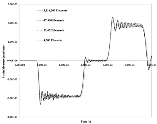
Figure 1: Plot of variation of incident and reflected strain measurements, from Finite Element Analysis (FEA), due to mesh refinement. The element type for this study was regular hexahedral. Four cases of mesh refinement, varying from 4,703 to 3,111,000 elements, were considered.

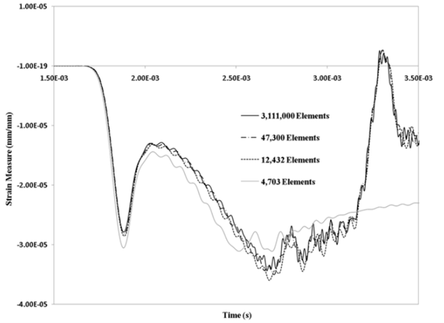
Figure 2: Plot of comparison of transmitted strain measures, from FEA analysis, due to mesh refinement. The element type considered for this study was regular hexahedral. Four cases of mesh refinement, varying from 4,703 to 3,111,000 elements, were considered.

A specific material model, MSU TP 1.1 (Bouvard et al., 2010)[2], was used to capture the elastic and inelastic response of the brain material. A summary of the constitutive equations is shown in Table 2.

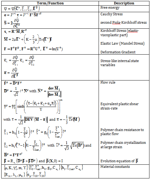
Table 1: Summary of the Model Equations for MSU TP 1.1 (see Bouvard et al., 2010[2])

The constitutive model ( MSU TP Ver. 1.1 ) presented in this paper captures both the instantaneous and long-term steady-state processes during deformation and could admit microstructural features within the internal state variables. With the microstructural features, we can use our internal state variable model so that eventually history effects could be captured and predicted. In the absence of the microstructural features, other constitutive models should be able to show the non-uniformity of the stress state under the high rate loadings exhibited here since no varying history was induced. Data from high strain rate tests were used to calibrate MSU TP 1.1 using a 1-D MATLAB (MathWorks Inc., 2010)[3] version of MSU TP 1.1(material point simulator). The model calibration was two-fold. The first step in calibration was performed such that the experimental and FEA strain gage data analyzed through MSU High Rate Viscoelastic software was in good agreement (Figure 4).

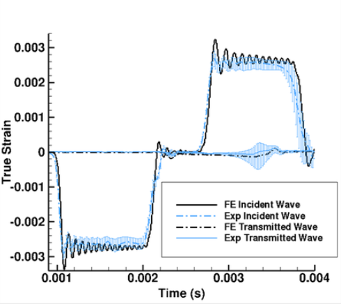
Figure 3: Comparison of experiment and Finite Element (FE) simulation σ₃₃ for porcine brain sample compression at 750 s^-1. FE simulation σ₃₃ were calculated by post processing the strain measurements from FE simulation through MSU High Rate Viscoelastic software

In the second step of calibration, the strain gage measurements from the SHPB experiment and FE simulation were also correlated. Figures 5 shows the comparison of the experimental and FE simulation strain gage data. The experimental and FE data have a strong correspondence. Thus, correlation was performed for both strain measurements and the stress-strain of the specimen. It is noteworthy here that the material point simulator, being1-D, gives a 1-D stress state for calibration; while the stress state in experiments and FE simulations is 3-D. The difference in the loading direction stress σ33 between the material point simulator, experiment and FEA is due to the presence of a 3-D stress state in the experiment and FEA (Figure 3,4 and 5 of Coupled Experiment/FEA Analysis).

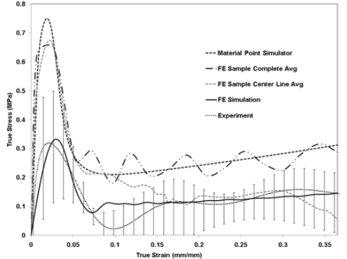
Figure 5: Comparison of incident, reflected and transmitted strain measurements in a Split-Hopkinson Pressure Bar (SHPB) for experiment and Finite Element (FE) simulation. The error bands in the experimental incident/reflected waves represent standard deviation.

So the model calibration was performed through an iterative optimization scheme where model constants were varied appropriately until the experimental and specimen volume averaged FE simulation σ₃₃ matched. The values for the material constants for MSU TP 1.1 are found in Table 3.

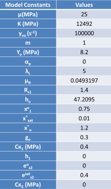
Table 2: Summary of the Model Equations for MSU TP 1.1 (see Bouvard et al., 2010[2])

Thus, FE simulations were usedin ABAQUS/EXPLICIT (Simulia Inc., 2009) to further analyze the different components of the stress tensor, similar to the way a specimen would undergo deformation during a SHPB experiment. Two specimen geometries were used for conducting FE simulations, namely cylindrical and annular. The annular specimen has an inner hole with a diameter that is 30% of the specimen diameter. The thickness of the cylindrical and annular specimens was 15 mm.

Reference

1. Simulia Inc., (2009), “ABAQUS/Explicit User’s Manual”, Version 6.9, Providence, RI, 02909, USA.

2. 2.0 2.1 2.2 Bouvard, J.L., Ward, D.K., Hossain, D., Marin, E.B., Bammann, D.J., and Horstemeyer, M.F., 2010, A General Inelastic Internal State Variable Model for Amorphous Glassy Polymers, ActaMech, DOI 10.1007/s00707-010-0349-y.

3. MathWorks, Inc. “The Language of Technical Computing”. At:http://www.mathworks.com/matlab, last accessed January, 2010.