


AFLR2C Example Cases
Data files for several AFLR2C sample cases are provided. Package
archives with all of the example cases are provided in
aflr2c-examples.tar.gz
(tar-gzip archive for Linux/MacOSX) and
aflr2c-examples.zip (zip archive for Windows).
Copy the package archive files and unpackage them in a location of your
choosing to run the example cases. All cases require minimal resources. The
input surface edge grid files provided for the sample cases are ASCII formatted
files of either BEDGE type or 2D FGRID type. In the following case examples the
output mesh file is a big-endian double precision C-binary (.b8) 2D UGRID type
file. Alternative file types can be used. By default the output volume mesh is
a big-endian double precision C-binary (.b8) 2D UGRID type file named
case_name.b8.ugrid. An isotropic element planar mesh can be generated for any
of the sample cases using the following command.
aflr2c -i case_name
See the AFLR2C documentation for information on
available options and usage. Alternatively you can view text-based documentation
at the command line with the following command.
aflr2c -help
The XPLT2 program is provided to visualize the mesh that is output from
AFLR2C. To display the output mesh using XPLT2 use the following command.
xplt2 case_name.b8.ugrid
Text-based documentation is available at the command line with the following command.
xplt2 -help
Several AFLR2C example cases are provided and described below.
Mesh between two circles
aflr2c -i circle

Quad/tria mesh between two circles
aflr2c -quad -i circle

Mesh in a box
aflr2c -i box

Quad/tria mesh in a box
aflr2c -quad box

Mesh around NACA0012 airfoil
aflr2c -i n12


Quad/tria mesh around NACA0012 airfoil
aflr2c -quad -i n12


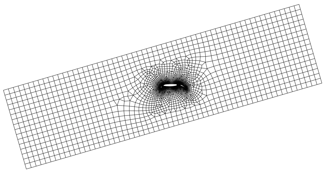
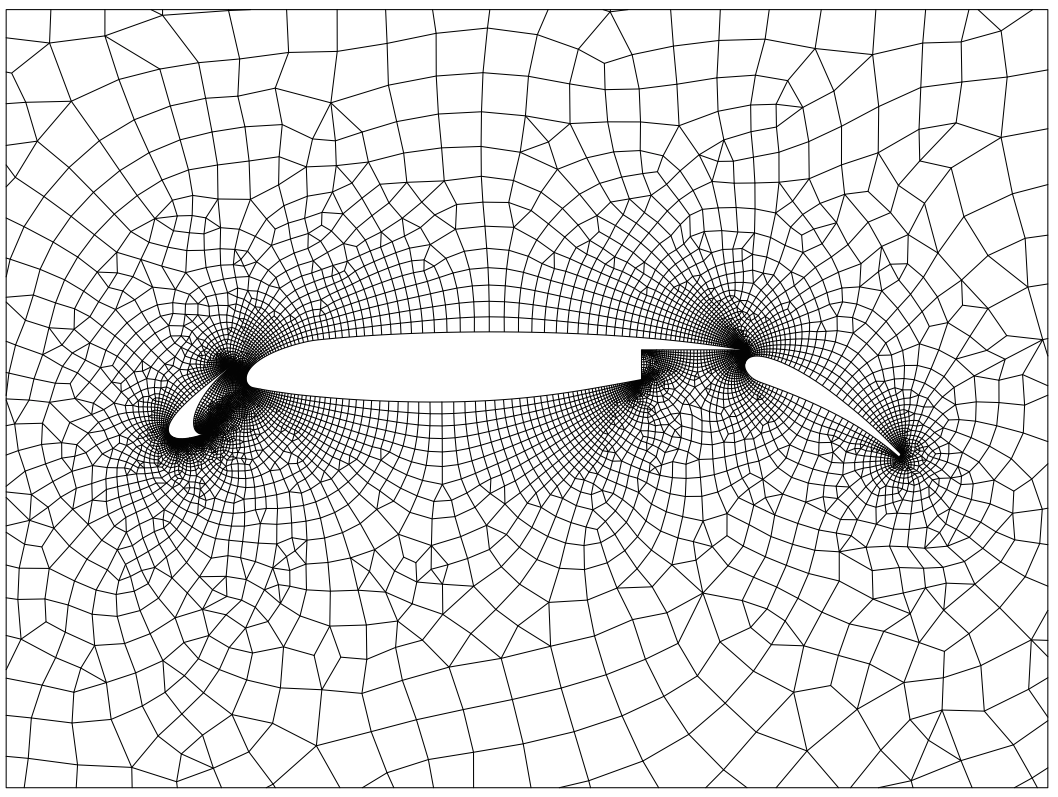
Mesh about a multi-element airfoil
aflr2c -i m3


Quad/tria mesh about a multi-element airfoil
aflr2c -quad -i m3
Mesh with multiple different inner and outer shapes
aflr2c -i shapes.fgrid

Quad/tria mesh with multiple different inner and outer shapes
aflr2c -quad -i shapes.fgrid

Mesh for Atlantic ocean with field growth
aflr2c -grow1 -i atlantic

Quad/tria mesh for Atlantic ocean with field growth
aflr2c -grow1 -quad -i atlantic

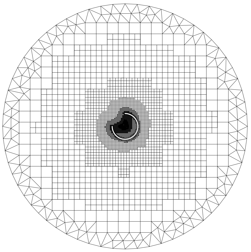
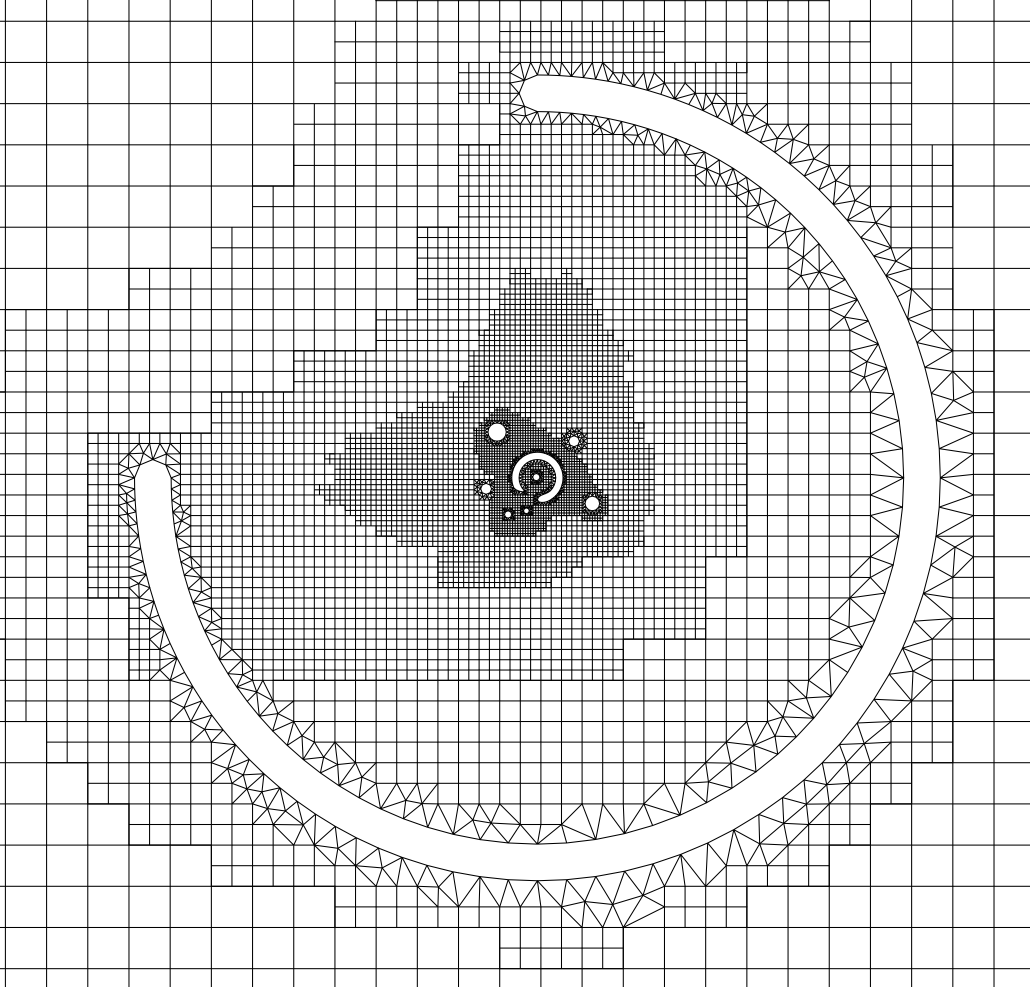
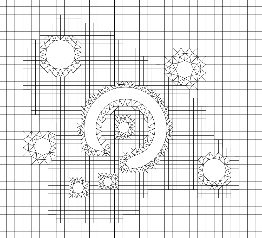
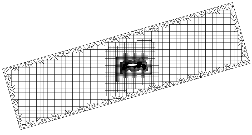
Quad/tria mesh for multiple objects with a quad interior core mesh
aflr2c -i things_ic_bnd -ice -o things_ic.b8.ugrid
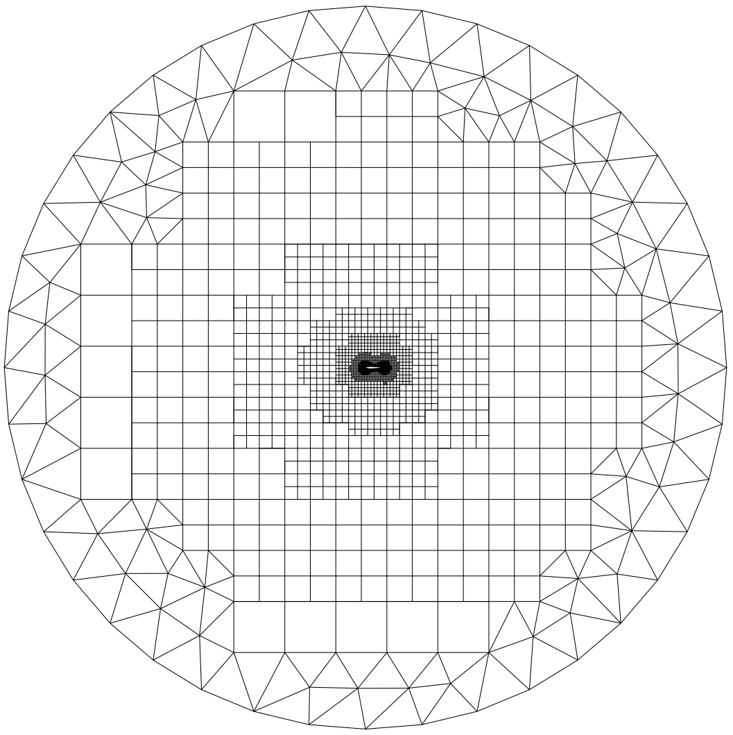
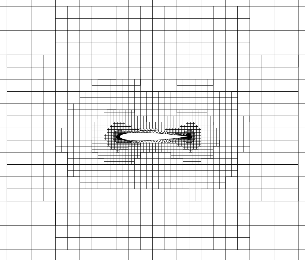
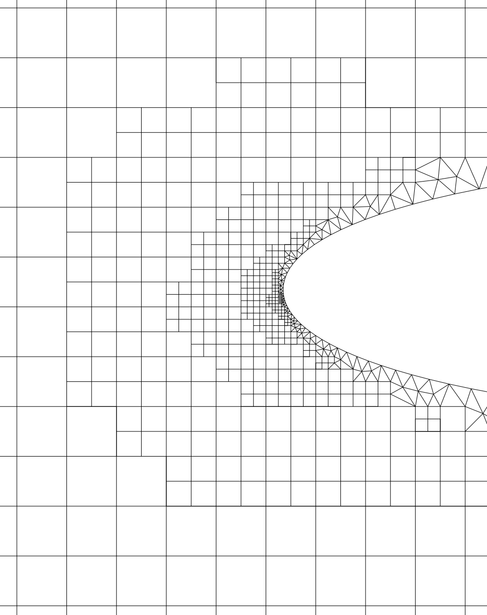
Quad/tria mesh around NACA0012 airfoil with a quad interior core mesh
aflr2c -i n12 -ice -o n12_v3.b8.ugrid
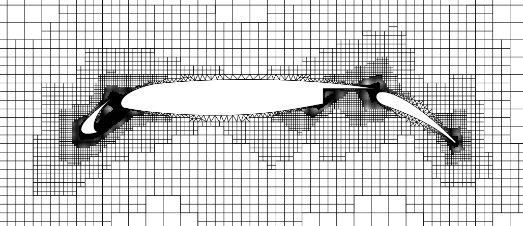
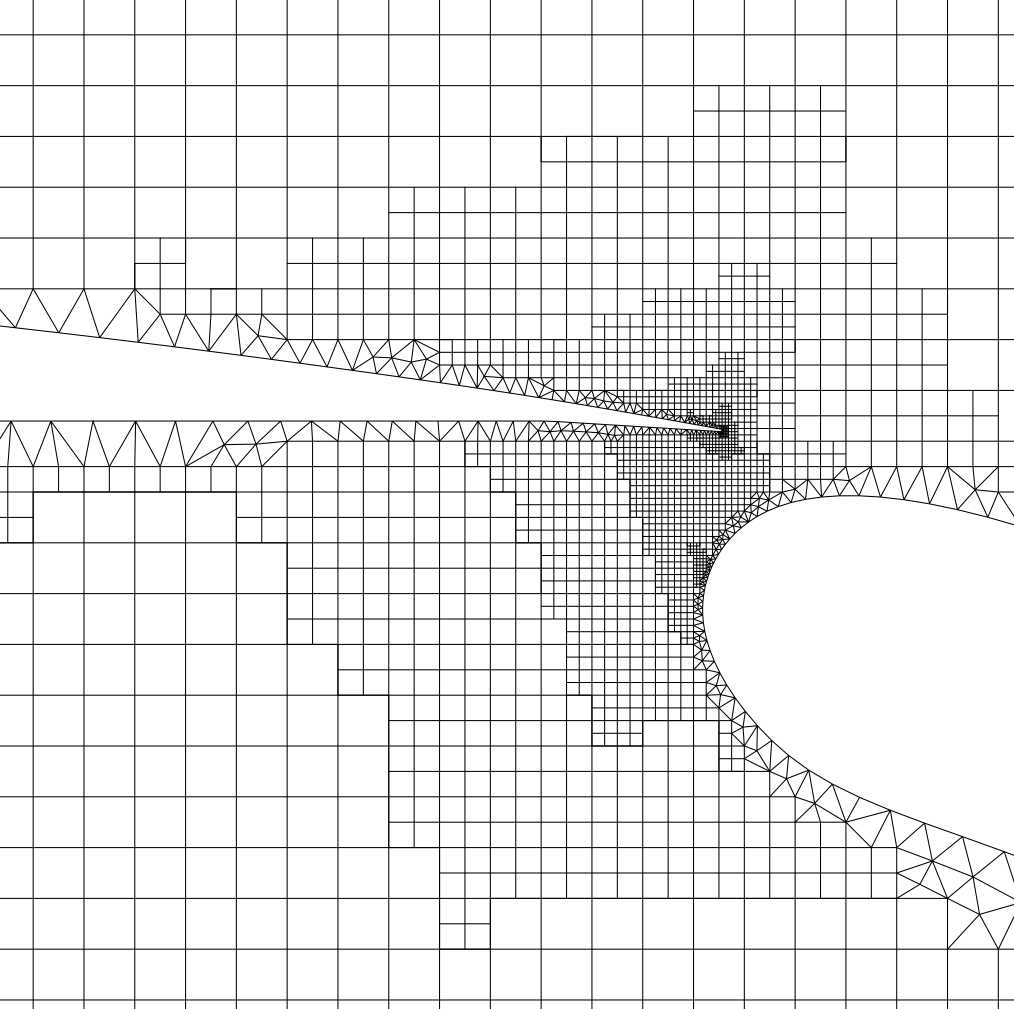
Quad/tria mesh around multi-element airfoil with a quad interior core mesh
aflr2c -i m3 -ice -o m3_v3.b8.ugrid
Mesh Sizing
In default mode AFLR2C determines element sizing based on interpolation between boundary points (and source points, if any). As mesh generation advances the sizing is propagated by continued interpolation locally. Alternatively, an external sizing function can be coded and linked with the executable. A built-in external sizing function is provided for testing and example. By itself it is not useful for practical problems. However, developers can integrate specialized sizing functions within the AFLR2C executable. The built-in function simply creates a continuous field that varies radially from the center of the domain outward to the boundaries. At the center the sizing is smaller than specified at the boundaries. Another alternative for sizing is to use a background mesh and function file for interpolation. If the files case_name.back.b8.ugrid and case_name.back.sfunc exist then it is assumed that use of a background mesh is desired. Note that any supported and readable mesh and function file format and type are equally as acceptable as .b8.ugrid and .sfunc. The case name case_name must be the same as the input surface mesh file. The option flag -no_back can be added to ignore these files.
Box with external isotropic sizing function
The following example uses
the built-in external sizing function. If an alternative routine is created
then use of that function can be controlled in the same manner or by using the
correct meval=# for the alternative function. The provided built-in sizing
function has test cases for meval=1,2,...6 (4,5,6 require use of a metric - see
next section). This case also creates a background grid sizing field that will be
used in the next case. The option flag meval=1 activates use of the alternative
built-in external sizing function #1 and the flag mwbgfunc=1 (not required for
normal usage) simply creates an output function file box.back.sfunc which
contains the isotropic sizing for each mesh vertex.
aflr2c -i box meval=1 mwbgfunc=1

Box with background mesh for interpolation of isotropic sizing
Another alternative for sizing is to use a background mesh and function file
for interpolation. If the files box.back.b8.ugrid and box.back.sfunc exist then
it is assumed that use of a background mesh is desired. Note that any supported
and readable mesh and function file format and type are equally as acceptable
as .b8.ugrid and .sfunc. The option flag -no_back can be added to ignore these
files. In this test case the background mesh sizing field is derived from the
previous case. It could also be generated from another code that bases the
sizing on the computed physics or other criteria. The resulting mesh is
equivalent to the previous case (on which it is based). However, it does differ
since here we are interpolating rather than determining the sizing
analytically.
cp box.b8.ugrid box.back.b8.ugrid
aflr2c -i box
Anisotropic Adaptation/Generation
In
default mode AFLR2C determines element sizing based on interpolation
between boundary points (and source points, if any). Alternatively, the sizing
can be interpolated from a background mesh. In addition, the background mesh
may specify, in a function file, either the isotropic mesh sizing or
directional metric based sizing. If the executable is able to find a set of
files named case_name.back.* for the background mesh that is a valid mesh type
file along with a background sizing function file that is a valid function file
then the background data will be read in and used. The case name case_name must
be the same as the input surface mesh file. The option flag -no_back can be
added to ignore these files. If the metric option is on (mmet=1 or 2) then the
function file must contain a metric for every background mesh vertex. And, if
the metric option is off (mmet=0) as it is by default then the function file
must contain an isotropic spacing for every background mesh vertex. With a
background mesh all element sizing is interpolated from the background mesh.
The first step in the mesh generation process in adaptation mode is a
regeneration of the input boundary edge grid. The vertex spacing on the
boundary edges is determined from the background mesh. Cubic splines based upon
the input boundary edge grid are used for geometric specification. As such, the
input boundary edge grid should be of sufficient resolution to resolve the
geometry. Splines are split between boundary edges of different IDs and at
discontinuities. The detection of discontinuities is controlled by the input
parameter angdbe (discontinuous boundary edge angle). If the angle between two
adjacent boundary edge vectors differ by more than angdbe then the location is
considered discontinuous. The discontinuity angle may need to be modified for
configurations that do not have differing boundary edge IDs and low-angle
discontinuities.
Subsequent mesh generation steps follow the normal process, except that sizing
is interpolated from the background mesh. With metric based adaptation/generation
it is recommended that right angle elements be used (mpp=3) as the point
placement strategy uses alignment with the background metric. Typically the
only option required is -met3 (mmet=1 mpp=3). Note that at present smoothing is
turned off when metrics are used.
Box with a cross
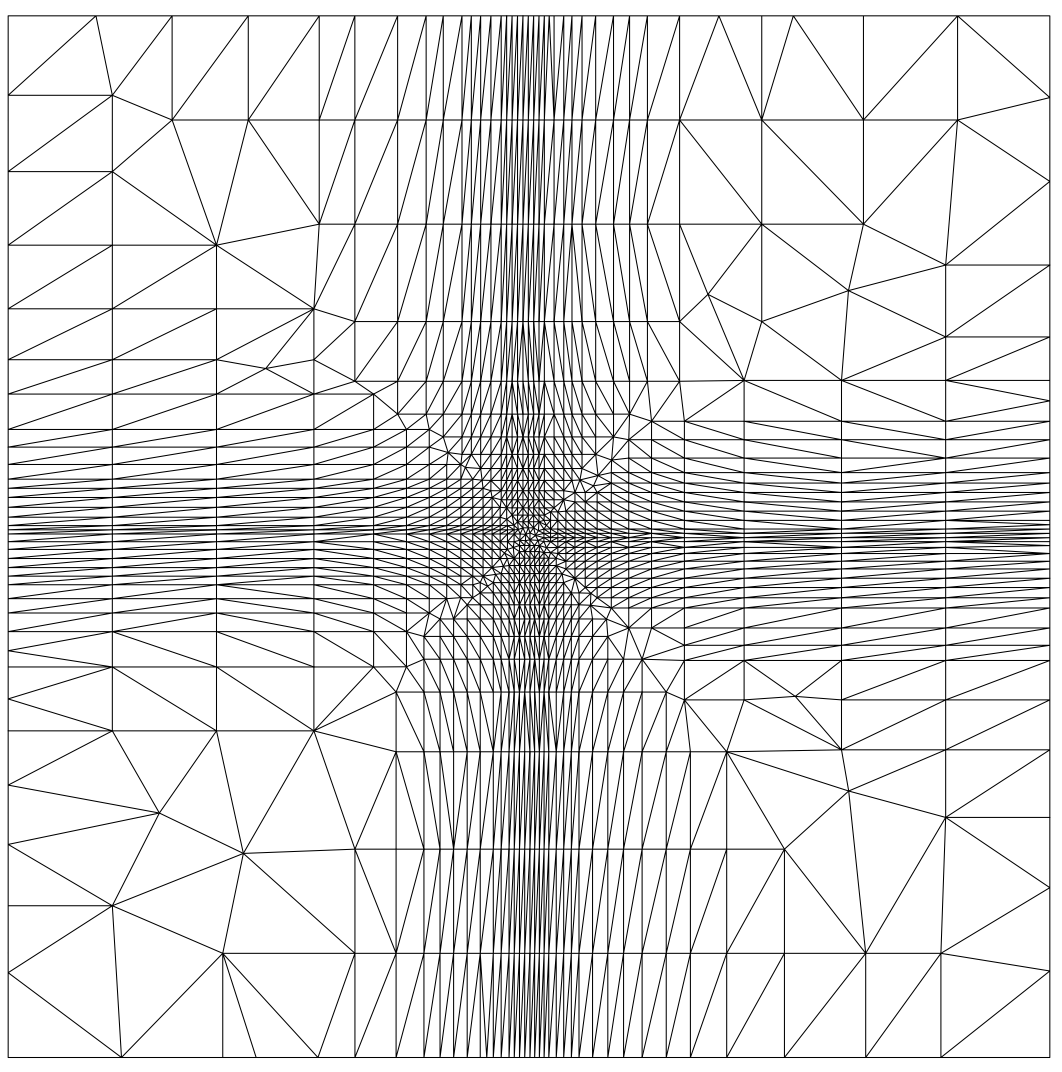
The following example uses the built-in external
sizing function and creates the metric field instead of using a background
mesh. If an alternative routine is created then use of that function can be
controlled in the same manner or by using the correct meval=# for the
alternative function. The provided built-in sizing function has test cases for
meval=1,2,...6 (4,5,6 require use of a metric - see next section). The option
flag met3 turns on use of the metric and right angle point placement and the
option flag meval=5 activates use of the alternative built-in external sizing
function #3 (blended cross).
aflr2c -i cross -met3 meval=5
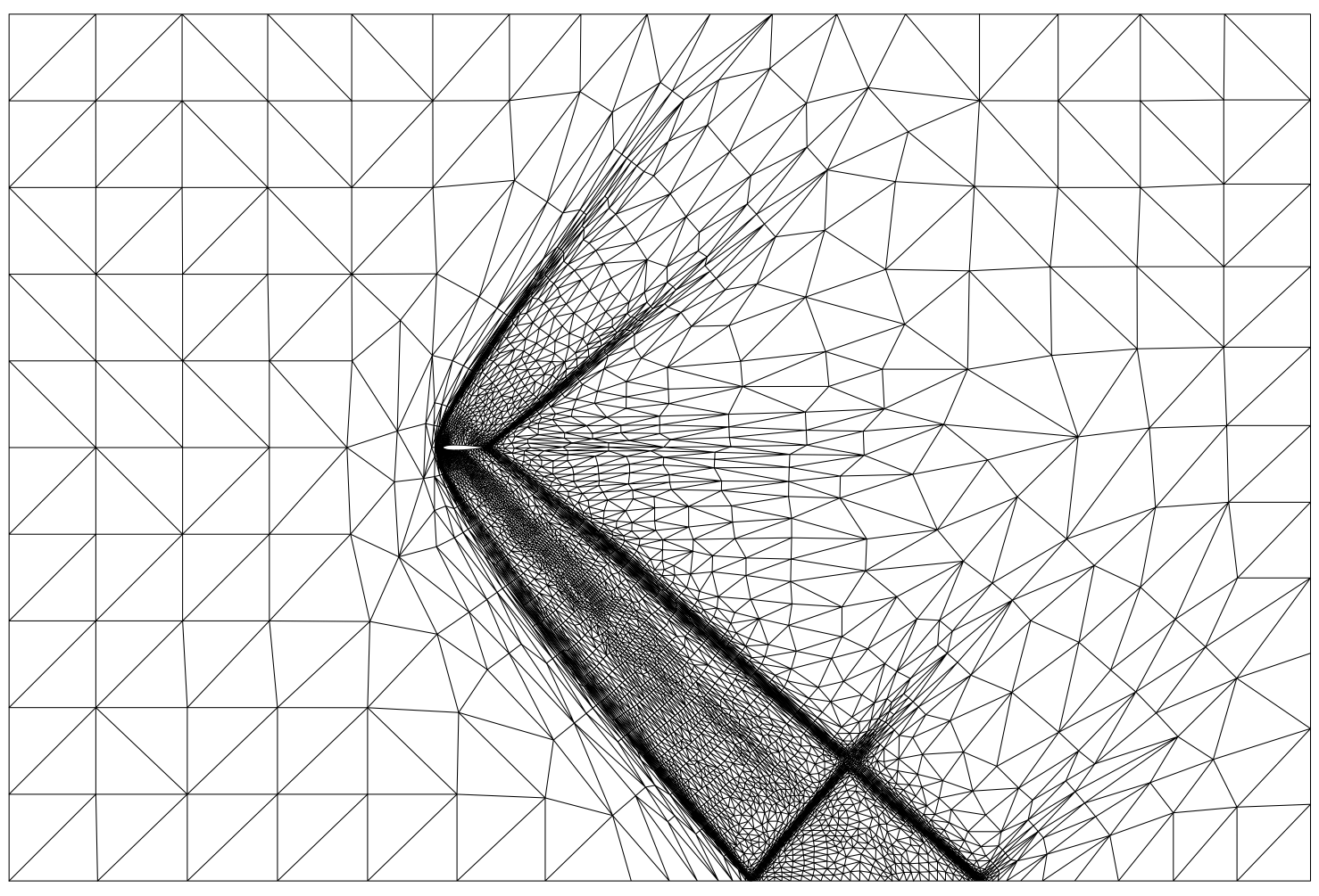
Supersonic NACA Airfoil
The following example for a NACA airfoil in a supersonic
flow field uses a supplied background mesh and metric field. The option
flag met3 turns on use of the metric and right angle point placement.
aflr2c -i naca -met3
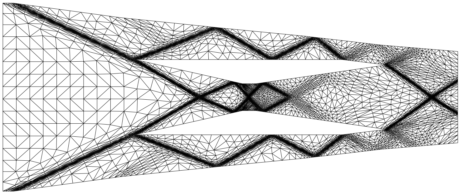
Scramjet
The following example for a scramjet field uses a supplied background mesh and
metric field. The option flag met3 turns on use of the metric and right
angle point placement.
aflr2c -i scramjet -met3
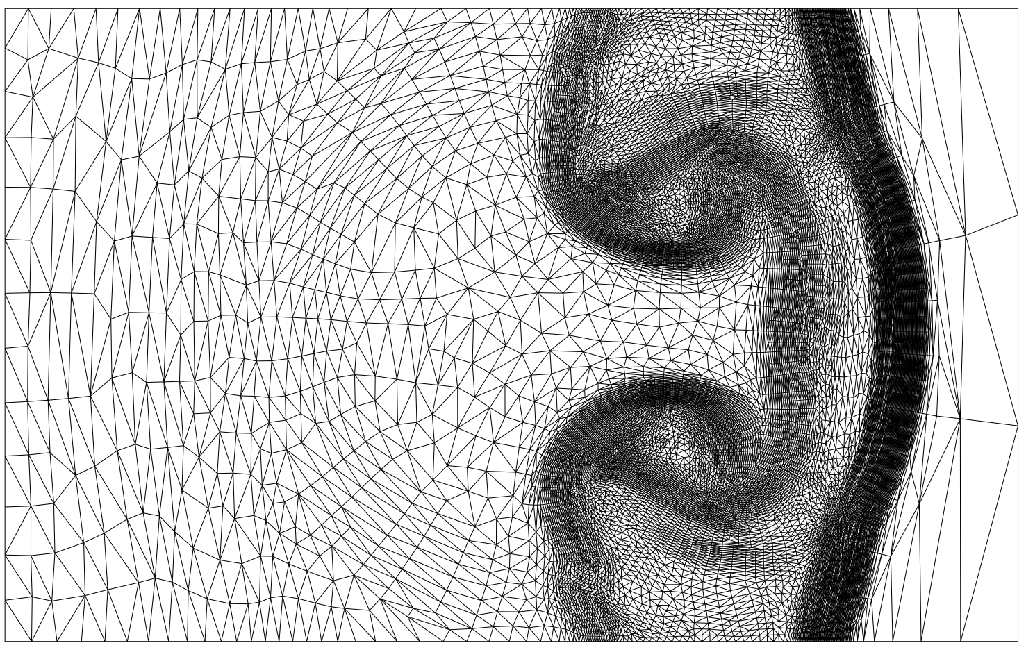
Shock Bubble Interaction
The following example for a shock interacting with bubble in a supersonic flow field uses a supplied background mesh and metric field. The option flag met3 turns on use of the metric and right angle point placement.
The BSURF2 program is also provided to generate boundary edge grid files
It is
an interactive program and the prompts should be descriptive enough to allow
usage. Package archives with example files for the BSURF2 code are
provided in bsurf2-examples.tar.gz
(tar-gzip archive for Linux/MacOSX) and
bsurf2-examples.zip
(zip archive for Windows).BSURF2 is not that well documented
and it would be much
easier to use in a GUI. However it gets the job done and is not that painful to
use. The objects in the geometry can be a circle, polygon, or come from a data
file. The data file must be a string of x and y coordinates (one set per line)
in sequential order that form a closed curve (do not duplicate the last data
point). The direction (clockwise or not) is not important. A spline is
generated for each object and automatically split at the first and last data
points and at detected discontinuities. Spline split points can be added or deleted.
A script file is created that allows one to rerun a case with a corrected error
or slightly different parameters. Edit the script file (default name is
bsurf2.script) to make changes and rerun BSURF2. The # comments should
provide information necessary to modify the right parameters. If you make an
error while running BSURF2 and want to start over from a previous point
in the session then kill the process. In this case edit the script file by
deleting everything from the point you made the unwanted step to the end of the
file. Then rerun BSURF2 using the script file you edited as the input
script file. The program will redo all the steps contained in the script file
and return standard input control to you when it reaches the end of the file.
To run BSURF2 in interactive mode simply enter the following and follow
the interactive prompts.
bsurf2
Note that BSURF2 generates ASCII formatted type BEDGE edge grid files.
These are exactly the same as the older, and now obsolete, BSURF type files
that older versions of BSURF2 generated. AFLR2C can input BEDGE,
BSURF, 2D FGRID or 2D UGRID file types. See the
UG_IO documentation for
a description of standard UG_IO file types used by AFLR2C.
BSURF2 example cases are provided and described below. The script files
for each are configured to generate a suitable boundary edge grid for AFLR2C.
Mesh around NACA0012 airfoil
bsurf2 n12
aflr2c -i n12
Mesh with multiple different inner and outer shapes
bsurf2 shapes
aflr2c -i shapes